Statistics

Statistics lies at the heart of decision-making across various fields of science and business. In risk management, it plays a pivotal role in helping companies quantify uncertainties, such as the probability of insolvency or the likelihood and magnitude of claims. By providing a framework to model and analyze risk, statistics forms the backbone of actuarial science and informs nearly all aspects of effective risk management. In this post, we revisit fundamental statistical concepts to refresh your understanding and highlight their importance.

Distributions in Statistics

Random Variable and Distribution

In elementary statistics, we have surely come across the random variable. A random variable (notation capital $X$, capital $Y$, etc.) can be seen as a random realisations (small $x$, small $y$) of something measurable. For example, the time needed to travel from A to B. Statistics tells us that such random variable has a distribution that tells us how random realisations of the random variable is spread.

Of course we should remember there will certainly be cases where realisations can be discrete or continuous. A discrete realisation can be number of claims per interval, while a continuous realisation can be something as time taken to travel. Hence, we see distributions that are continuous or discrete.

Distributions can be described by this set of default matrics that is the mean and variance. The mean tells us the average values of the random realisations, while the variance tells us the spread of such random realisations from the mean. However, we will come to see that not all distributions directly have these parameters.

A very common continuous distribution out there is the Normal Distribution. The Normal distribution tells us directly that some random variable is distributed with some arbitrary mean $\mu$ and some arbitrary standard deviation $\sigma$. A common discrete distribution is the Poisson distribution that has a lambda parameter. The $\lambda$ parameter tells us the expected rate of which an event (that is Poisson distributed) occurs at some fixed interval. In this case we are not explicitly given the mean and variance, but the mean and variance can be found using the $\lambda$. Lambda of $5$ essentially tells us that the average of the different realisations of the Poisson distributed random variable will be 5.

Every random variable that has a distribution will have these probability metrics: the probability density function (pdf), the cumulative distribution function (cdf), and the quantile function.

In R, distributions are given different codes. These codes are imperative in order to execute R functions of the pdf, cdf, and the quantile. For instance, a Poisson distribution is noted as pois in R. The Normal distribution is noted as norm in R. To know more about the distribution codes in R, execute the command ?distribution.

Probability Density Function (pdf)

The probability density function (pdf) is a function that gives us the probability mass of a random variable $X$ taking on some realisation $x$, $X=x$.

\[P[X=x] = pdf(x)\]

In Rstudio, the function to find the density function is d«distribution code». It can be dnorm(), dpois(), et cetera.

# Find probability of a realization of 8 in a Poisson distribution with lambda 5
dpois(8, lambda=5)
[1] 0.06527804

#To visualise the pdf of the Poisson distribution of lambda 5, we can do as follows:

Cumulative Distribution Function (cdf)

The cumulative distribution function is the function that gives us the probability mass of a random variable $X$ being less than some realization $x$, $X<x$.

\[P[X < x] = cdf(x)\]

In Rstudio, the function to find the density function is p«distribution code». It can be pnorm(), ppois(), et cetera.

# Find probability of that a realization is less than 8 in a Poisson distribution with lambda 5
ppois(8, lambda=5)
[1] 0.9319064

Quantile Function

The quantile function on the other hand is the inverse of the cdf function. It basically finds the realisation as a threshold for which a given percentage/quantile (p, which we set) of realisations falls below it.

\[\text{Quantile Function} = \text{cdf}^{-1}(x)\]

In Rstudio, the function to find the quantile function is q«distribution code». It can be qnorm(), qpois(), et cetera.

# Find the realisation (threshold) for which 70% of the observations of Poisson distribution of lambda 5 lie below this threshold.
qpois(8, lambda=5)
[1] 6

Generating Realisations of some Distribution in R

We can use the function of r«distribution code» to generate realisations of some code. It can be rnorm(), rpois(), et cetera. The

#Generate 1000 realisations of a Poisson random variable with lambda 5
set.seed(10) #Ensures the command below generates same results
rpois(n=5, lambda=5)
[1] 5 4 4 6 2 3 4 4 5 4

Visualising the Univariate pdf and cdf of Continuous and Discrete Functions

Visualising graphs of the pdf and cdf are equally important. They allow us to see how the probability function develops as the realisations changes.

#First, we need to generate realisations (1000 of them) of a Normal(0,1) distribution (Continuous)
set.seed(100)
# Generating more realisations (1000) will give a more accurate x-range to work with later on.
gen_norm <- rnorm(1000, 0, 1)

#We make use of our realisations to findthe range of x values that we can generate to build the pdf and cdf graphs #of Normal(0,1) using the histogram function, that way we ensure a accurate pdf and cdf graph (to the tails of the #distribution) is shown.
hist(gen_norm) 

#We see that the realisations of a Normal distribution therefore lies between -3 and 3. These can be used
#to construct the sequence of x-values to use for the pdf and cdf graphing. I am not going to show the picture. Reader can confirm by using the code by oneself.

#Start coding inputs for the pdf graph
x_val <- seq(-3,3, length.out=50) #Create x-values sequence to input into the pdf function
pdf_val <- dnorm(x_val, 0, 1) #Returns values of pdfs for every x value (realisation) input
plot(x_val, pdf_val, type="l")
cdf_val <- pnorm(x_val, 0, 1) #Returns values of cdfs for every x value (realisation) input
plot(x_val, cdf_val, type="l")
abline(h=1, lty=3); abline(h=0, lty=3) #Visual barrier to tell us that CDF graph lies between 0 and 1 

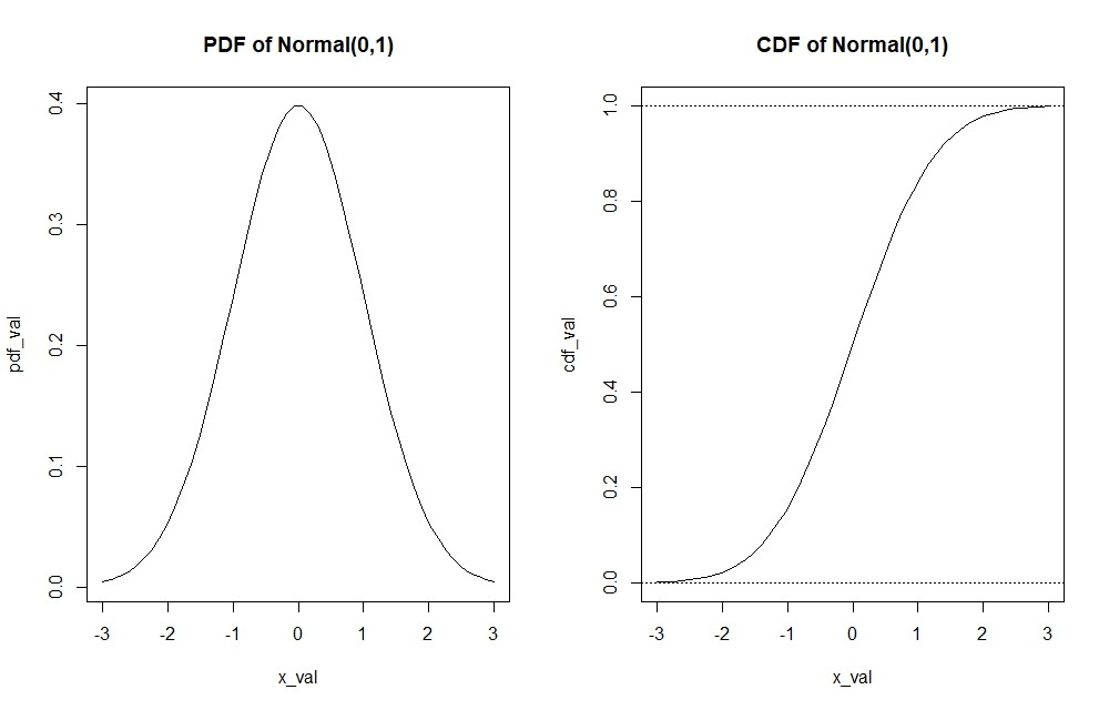
We can see for instance through the pdf function, which realisation holds the most probability mass in the $Normal(0,1)$ distribution or how the tails of the distribution look like. On the other hand, the cdf function allows to find important quantiles of the distribution.

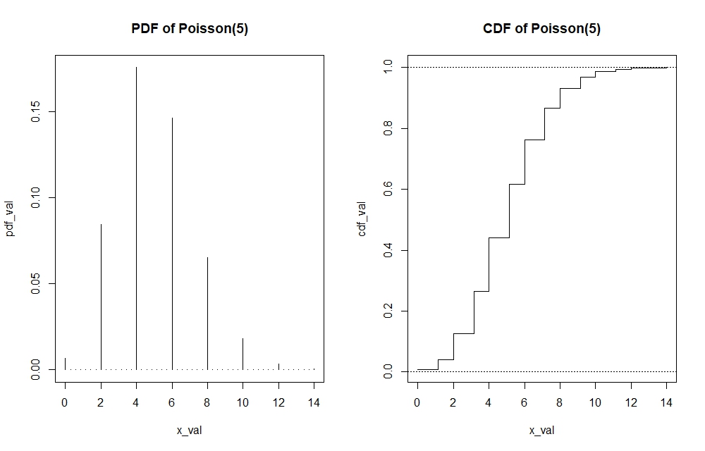
Note that I have graphed a continuous distribution above. If the distribution is discrete, then the pdf and cdf’s functions cannot be presented by straight line. In the case of the cdf of Poisson, the graph would look like a step function. In the case of Poisson pdf, the graph would look more like a histogram. Making these plots can be done by adding the argument of $type=”s”$ and $type=”h”$ in the $plot()$ function of the cdf and pdf respectively. I will show the visualisation of the Poisson(5) pdf and cdf. Since the code is rather repetitive, I will directly show the graphs while the code will still be available in the R-file itself.

Multivariate Distributions and Some Useful Commands in R

The concepts that we dealt above was in the univariate case, which means we are only dealing with one random variable. However, we should know that in reality it is not as simple as that. Take for instance in risk management, we expect to deal with multiple random individual claims in a portfolio, that can be $X_1$, $X_2$ up to $X_n$ where each belongs to some distribution. This requires we know joint distribution of all those random variables to be able to calculate metrics such as the pdf, cdf, quantiles related to these random variables.

Let us take a multivariate normal distribution as an example and compare it to its univariate counterpart to see the differences.

We need to note some changes to elements of the multivariate normal distribution versus the univariate normal distribution. While we dealt with only single values of mean and variance to describe the normal distribution in the univariate model. However, we now deal with vector of means and a variance-covariance matrix to describe distribution in the multivariate model. This should be logical as we assume every random variable possesses it’s own mean, hence the vector of means. We also assume by default that there is correlation between these random variables, and these are used to calculate the variance and covariances between variables that belongs in the variance-covariance matrix. Unless stated otherwise where there is no correlation between variables, covariances between random variables are esentially zero leaving us a diagonal variance matrix only consisting of variances of every random variable on the diagonals.

To help visualise:

Univariate Normal Distribution pdf that requires only one mean ($\mu$) and one variance ($\sigma^2$) with a single number input $x$.

\[f(x) = \frac{1}{\sqrt{2\pi \sigma^2}} \exp\left(-\frac{(x - \mu)^2}{2\sigma^2}\right)\]

Multivariate (n) Normal Distribution pdf which requires multiple means stored as a vector (bolded $\mu$) and multiple variances and covariances stored as a variance-covariance matrix (bolded $\Sigma$) with potentially multiple inputs of $x_1$, $x_2$ until $x_n$ as a vector (bolded $x$).

\[f(\mathbf{x}) = \frac{1}{(2\pi)^{n/2} (\det \boldsymbol{\Sigma})^{0.5}} \exp\left[-\frac{1}{2} (\mathbf{x} - \boldsymbol{\mu})' \boldsymbol{\Sigma}^{-1} (\mathbf{x} - \boldsymbol{\mu})\right]\]

To illustrate how to use the built-in multivariate function in R, I attempt calculate the bivariate normal pdf (as a case of the multivariate distribution) in R for the realisations $X=1$ and $Y=1$, using the function dmnorm(). In other words we aim to find $P[X = 1 , Y = 1]$.

# First, we construct the mean vector and variance-covariance matrix of the bivariate normal distribution
mean_vecx<-c(2,5) # mu
varX<-4; varY<-16; corXY<-0.1
covXY<-corXY*(varX*varY)^0.5
covar_matx<-matrix(c(varX,covXY,covXY,varY),2,2)

#Now, we want to find the probability of X=1 and Y=1
input_vector <- c(1,1) #Inputs of realisations x=1 and y=1 for the pdf 
dmnorm(input_vector, mean_vecx, covar_matx) #Finds the pdf of P[X=1, Y=1]
[1] 0.0111859

We can also find the cdf of multivariate distributions using pmnorm(), which we can see as the joint probability that $X$ lies below some realisation $x$ and $Y$ lies below some realisation $y$, that is $P[X<x , Y<y]$. We can also generate realisations of the bivariate distribution using rmnorm(). This command will generate some number of realisations of every random variable in the multivariate distribution by columns. One can try to practice by finding pdf’s and cdf’s of higher variate distributions, for instance of 3 random variables.

#Find the cdf of a bivariate normal distribution with same input, that is P[X<1. Y<1]
pmnorm(input_vector, mean_vecx, covar_matx)
#Set number of simulations and set.seed() to ensure you produce same results
set.seed(110); number_sims <- 15
rmnorm(number_sims, mean_vecx, covar_matx)

Creating pdf and cdf graphs of the bivariate normal distribution (as a case of the multivariate distribution)

It is equally important to know how to graph the bivariate pdf and cdf. The purpose of illustrations remain the same as in the univariate case, to understand important data points that give the most probability mass and to identify important quantiles of the distribution. Below is the code to do so.

# Create pdf and cdf graphs of bivariate normal of the same parameters above
number_sims_new <- 1000
gen_biv <- rmnorm(number_sims_new, mean_vecx, covar_matx)
hist(gen_biv[,1], main="Spread of Random Variable X"); hist(gen_biv[,2],main="Spread of Random Variable Y")

#We see that for X, realisations lie between -4 and 8, while for Y, realisations lie between -5 and 20.

x_biv <- seq(-4, 8, 0.5); y_biv <- seq(-5, 20, 0.5)

#Create pdf function that allows us to input x and y realisations into the multivariate pdf 

pdf_biv <- function(x,y){dmnorm(cbind(x,y), mean_vecx, covar_matx)}
cdf_biv <- function(x,y){pmnorm(cbind(x,y), mean_vecx, covar_matx)}

# Now, we need to find values of the pdf for every different possible combinations of the x and y
# The function outer() does the trick for us. 

pdf_valbiv <- outer(x_biv, y_biv, pdf_biv)
cdf_valbiv <- outer(x_biv, y_biv, cdf_biv)

# The pdf we plot now is essentially a three dimensional plot, which we can display either 3-dimensionally by 
# a perspective plot persp() or a 2-dimensional contour plot
par(mfrow=c(1,2))
persp(x_biv, y_biv, pdf_valbiv, xlab="x", ylab="y", zlab="Bivariate PDF", main="Bivariate PDF Perspective plot")
contour(x_biv, y_biv, pdf_valbiv, xlab="x", ylab="y", main="Bivariate PDF Contour plot")
par(mfrow=c(1,2))
persp(x_biv, y_biv, cdf_valbiv, xlab="x", ylab="y", zlab="Bivariate CDF", main="Bivariate CDF Perspective plot")
contour(x_biv, y_biv, cdf_valbiv, xlab="x", ylab="y", main="Bivariate CDF Contour plot")

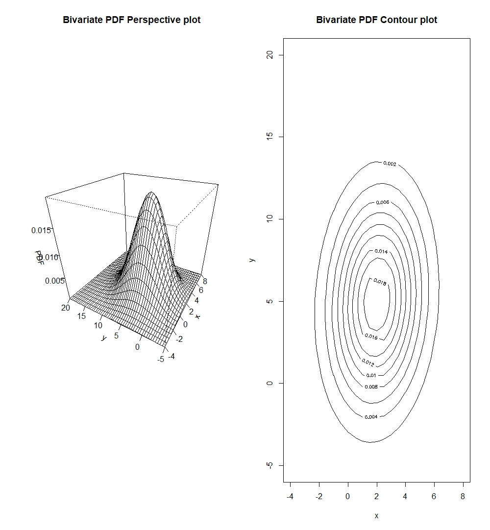
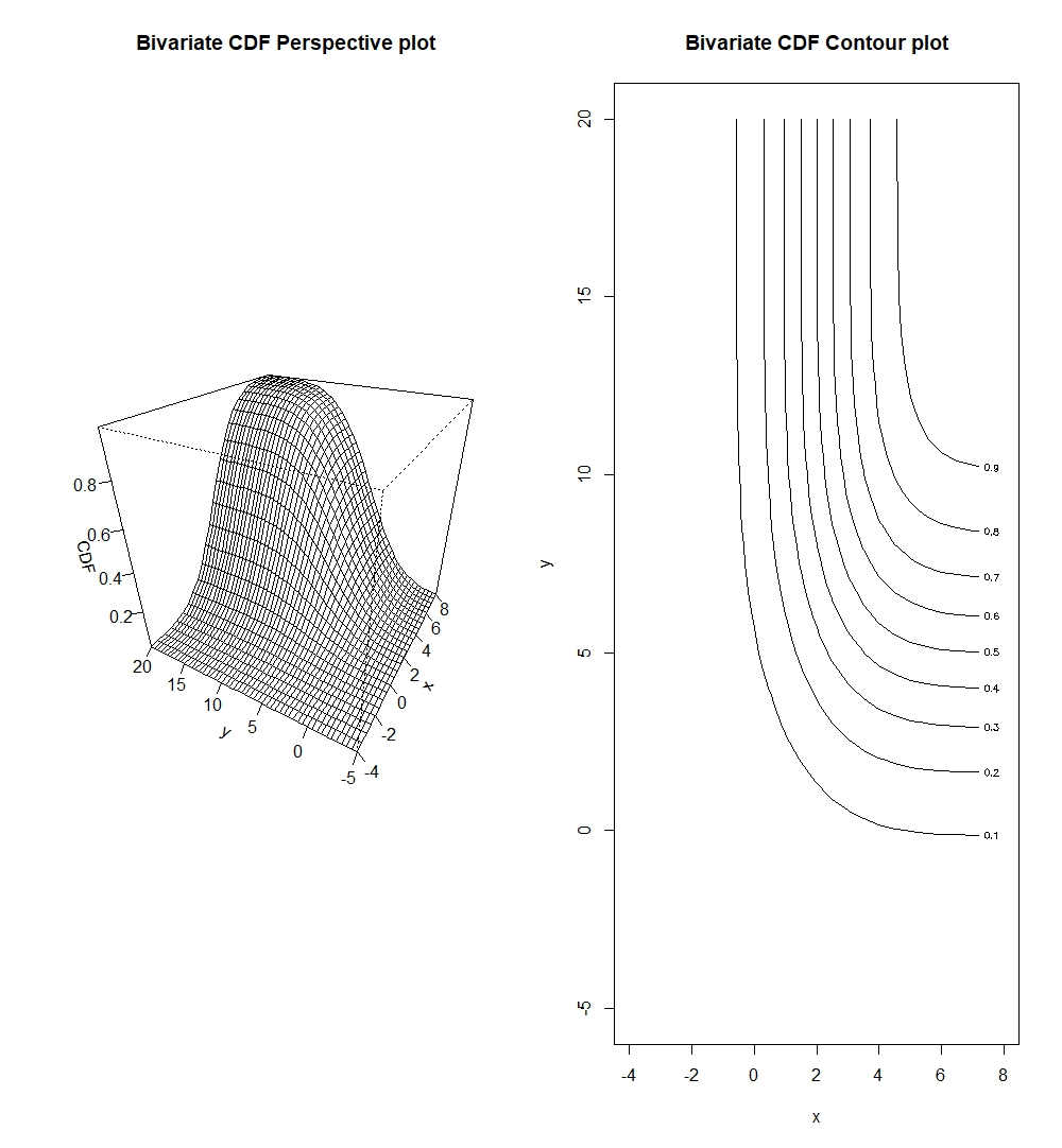
We should note that contour plots are esentially horizontal slices of the perspective plots.

One might ask whether it is possible to plot all dimensions of a multivariate probability function. Unfortunately, a larger dimensional graph (say n+1 dimensions) would not be handy as it would be hard to interpret. Thus, most people use at most 3 dimensional graphs to illustrate relatonships of bivariates. If one is presented with a tri-variate distribution (three random variables) or further, then it is best to plot different bivariate combinations of the trivariate (or multivariate) distribution. This is still useful to us as pairwise plots of the three (or multiple) variables can allow us to potentially identify dependencies of these variables while marginalising the others.

There are more R-packages that contain built-in functions for different multivariate distributions. The reader is encouraged to explore these further.

Descriptive Statistics

Descriptive statistics as we will see below can be very useful to show distributions of single variables and the pairwise descriptive statistics and visualisations of multiple variables.

summary() Function

We can use the summary() function in R to look at important descriptive statistics. This function produces a list of important descriptive statistics that can inform the user on how the dataset is distributed. Let us take a summary of the $\text{Trees}$ base dataset in R.

library(datasets) #install.packages("datasets") if not yet installed
trees #trees dataset is base dataset, there is no need to load it, simply typing trees will show
colnames(trees)[1] <- "Diameter" # change column name from "Girth" to "Diameter"
summary(trees)

    Diameter    Height       Volume     
 Min.   : 8.30   Min.   :63   Min.   :10.20  
 1st Qu.:11.05   1st Qu.:72   1st Qu.:19.40  
 Median :12.90   Median :76   Median :24.20  
 Mean   :13.25   Mean   :76   Mean   :30.17  
 3rd Qu.:15.25   3rd Qu.:80   3rd Qu.:37.30  
 Max.   :20.60   Max.   :87   Max.   :77.00  

The summary gives us important statistics such as the minimum and maximum values of the variable in the datasets, and important quantiles.

To find the most common descriptive statistics of mean, variance, correlation in R, we can use mean(), var(), and cor().

Scatter Plots and Pairwise Plots

There are also functions that can help visualise distributions of the data.

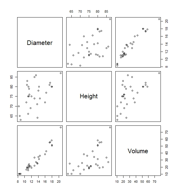
Take for instance the built-in functions of plot() which gives us the scatter plot between Diameter, Height and Volume. Via this scatterplot we will be able to deduce important relationships of variables. For instance, we can see that there is a fairly high positive correlation between the variable Diameter and Volume simply by looking at the plots below without having to know the precise correlation coefficient.

#Pairwise scatter plots of all variables in the trees data
plot(trees)

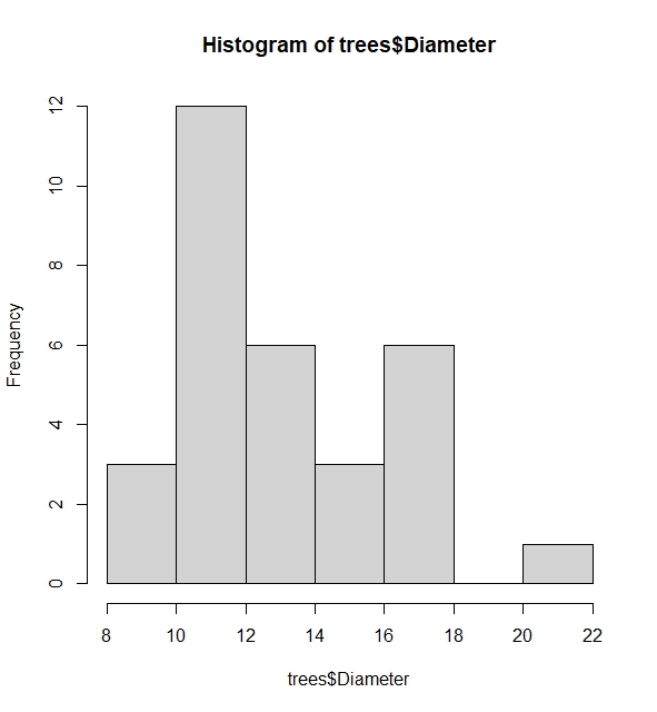
Another useful function is the histogram. This allows us to see the spread of a variable. We can use hist(). Let us find the histogram of the variable Diameter in the trees dataset.

# The histogram shows spread using frequency or probabilities (when freq=FALSE added)
hist(trees$Diameter, freq=FALSE) 

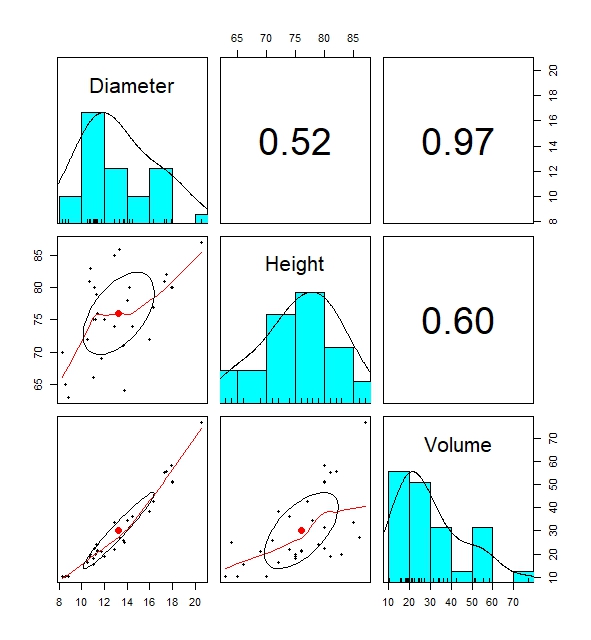
The most informative built-in function for descriptive statistics is the pairs.panels() data. The built-in function creates pairwise plots of regression lines, histogram and correlation coefficients of variables in the data that shows the relationship between variables in a data which can be useful.

# Pairwise plots shows distribution of dataset by displaying numerous descriptive statistics visualisations
pairs.panels(trees)

This is everything so far on basic descriptive statistics. Of course, there are more built-in functions out there which I might not have discussed. It is always wise to explore those further.

Hypothesis Testing: The Basis to all Statistical Tests

A hypothesis that states something about a population is true or not. If a hypothesis is not true, there should be an alternative hypothesis. Therefore through hypothesis testing, we attempt to either accept one hypothesis while rejecting the other. We normally call the two hypotheses as the null hypothesis and the alternative hypothesis.

This is done by incorporating statistical tests that can help aid in forming such conclusion. Of course, there is a chance that we do not arrive at the correct conclusion, such as when one rejects the null hypothesis given the null hypothesis is true, or accepting the null hypothesis when the null hypothesis is false. This is called the type I error and type II error respectively. A $\text{type I error}$ is considered to be more serious than a $\text{type II error}$, hence statistical testing is based on trying to limit the probability of making a $\text{type I error}$ to some level called the significance level ($\alpha$).

p-value as a Statistical Concept for Statistical Testing

In elementary statistics classes, you might have learned statistical testing by first determining some significance level, then constructing some rejection region based on that significance level that can reject the null hypothesis, before calculating some test statistic based on observed data which we check lies in the rejection region or not. If the test statistic lies in the rejection region, we reject the null, otherwise, we accept the null.

However, most built-in hypothesis testing functions in statistical softwares do not show rejection regions. Rather, they produce quick ouputs of some test-statistic with it’s associated p-value which we can directly compare to some significance level to conclude the hypothesis test. It is not to say that knowing how to find rejection regions is unimportant, but I will only be focusing on the p-value in this article due to it’s popular use in softwares. The reader can do self-study on how rejection regions are constructed.

The p-value tells us the probability of obtaining a test statistic more extreme (and/or equal) than what is observed (from the data we use for hypothesis testing), given that the null hypothesis is true and this serves as evidence against the null hypothesis.

\[\text{p-value} = P[\text{Test statistic} \geq x | \text{H_0 true}]\] \[\text{p-value} = P[\text{Test statistic} \leq x | \text{H_0 true}]\]

Determining which extreme tail it is ($\geq$ or $\leq$) requires that we understand the alternative hypothesis. If the alternative hypothesis deems that a population mean is lower than some value, then in order to reject $H_0$, we need to show probability of the observing an even lower sample mean than on our observed data given the null hypothesis to help with “finding” the evidence against the null.

Interpreting the p-value

The p-value can be seen as evidence to reject the null hypothesis. Looking at it’s composition, it esentially attempts to find whether the test statistic based on your observation (and it’s extremes) is likely under the null hypothesis. In practice, the lower the p-value, the more credible the evidence is to reject the null. But one can wonder, how does a low p-value serve as evidence?

Below I present two differing arguments to why we can use or not use this low p-value to conclude hypothesis testing.

• Can this directly considered evidence against the null? A small p-value could mean that our observations still fit the distribution under the null. It could simply be coincidence that we drew extreme observations under the null distribution for the test, but it does not necessarily mean that the null doesn’t explain the observations.
• On the other hand, if our test observation is extreme, then it can also be evidence that perhaps the observations is not best explained by the null. If the null were true, we expect our observed test statistic to fall in the high probability region of the null distribution (close to the mean).

This argument is broken by explaning the essence of hypothesis testing, which tells us that it is more “probabilistically” reasonable to believe that the null hypothesis is wrong than to believe that we have observed something extreme and improbable, hence it’s usage of a low p-value as evidence against the null.

“Evidence” does not tell us that the null hypothesis is $100$ percent false, simply that the evidence we received (based on observed data) shows that it does not reasonably fit the null hypothesis.

Linking the p-value to the significance level

So the question now is what is a maximum p-value that can be seen as enough to reject the null hypothesis?

Significance level comes into play here. In most literature, a $5$% significance level is deemed enough to draw a conclusion. In other words, if the p-value of obtaining an equal or more extreme test statistic than observed is less than $5$%, then we say we have sufficient evidence to reject the null hypothesis.

The significance level also acts as a barrier for the type I error. A more lower significance level (typically applied when deciding critical decisions) means that we are much more stricter in avoiding a type I error (rejection of the null hypothesis when the null hypothesis is true i.e. false positives), however there is also a trade-off that such low significance levels makes it more likely that null is not rejected and potentially miss out on detecting true effects.

Types of statistical tests

There are several common statistical tests out there. I will attempt to elaborate some of the important ones.

Normality Tests

Tests are normality are very common on statistical literature. This is necessary because conducting t-tests and variance tests (explained below) will require assumption that the data in question is normally distributed in order to produce accurate statistical inferences.

Common causes of non-normality can be when data is skewed heavy to one side, or when there are many outliers outside typical ranges in the data. Testing for normality can be done graphically or analytically. Each method can yield different conclusions on the normality.

Testing Normality Graphically

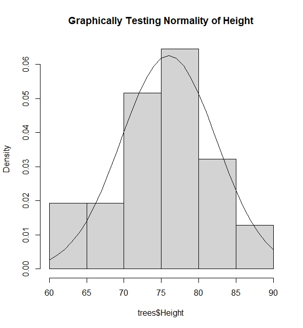
I give an example where I test if the the variable $\text{Diameter}$ in dataset $\text{Trees}$ is normally distributed via superposing the normal pdf function using mean and variance of variable above into the histogram of the variable.

#Find mean and variance of the variable Height assuming it has normal distribution
mh <- mean(trees$Height); vh <- var(trees$Height)

#Graph the spread of the variable Height
hist(trees$Height, freq=FALSE, main="Graphically Testing Normality of Height")

#We see that height takes value from 60 to 90, thus we try to find pdf of these height values assuming
#height is normally distributed

lines(60:90, dnorm(60:90, mh, sqrt(vh)))

#The histogram and the pdf clearly tells us that Height is normally distributed via this method as the spread
#of the Height fits the pdf of the height assuming it was normally distributed with some mean and variance.

Another method is to use the Normal QQ-Plot. The qqnorm() function plots the points of quantiles based on the given data of the variable, while the qqline() plot draws a line connecting the theoretical quantiles of the variables if it were normally distributed with mean and variance based on the data of the variable.

#Using QQ-plot
par(mfrow=c(1,3))
qqnorm(trees$Height, main="QQ Plot Height"); qqline(trees$Height)
qqnorm(trees$Diameter, main="QQ Plot Diameter"); qqline(trees$Diameter)
qqnorm(trees$Volume, main="QQ Plot Volume"); qqline(trees$Volume)

The deciding factor here to see whether such variable is normally distributed, is to see whether quantile points from the sample coincides with the theoretical quantile line. If quantile points from the data is close to the theoretical line, then it is enough evidence to suggest that the variable is normally distributed.

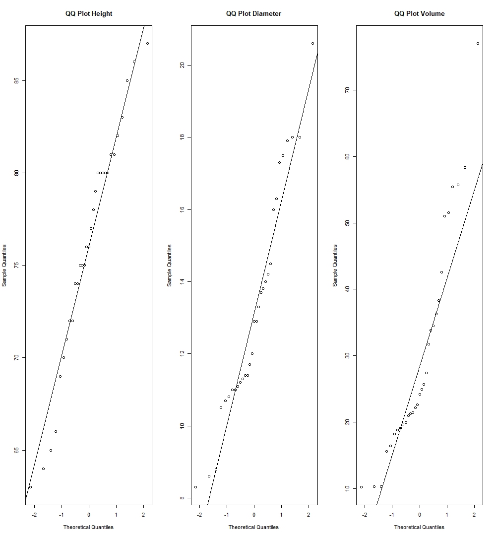
We can see by this method, we have strong evidence to suggest Height normally distributed as it’s sample quantiles lie very close to the theoretical quantiles, while there can be reasonable view to put into doubt whether Diameter and Volume are also normally distributed, as we see couple of deviations in the quantiles of these variables compared to the theoretical quantiles.

Testing Normality Analytically

There are various analytical tests for normality. They are to be found in the package $\text{nortest}$ in R. Some examples are the Jarque-Bera Test (used when observations are large), the Shapiro-Wilk and Anderson-Darling Test (used when observations are small). Here we assume that the null hypothesis states a variable is normally distributed, while the alternative is that it is not normally distributed. I will show whether the variables in the $\text{Trees}$ dataset are distributed normally via the R-code below:

#Jarque Bera Test
library(nortest)
library(tseries)

jarque.bera.test(trees$Height); jarque.bera.test(trees$Diameter); jarque.bera.test(trees$Volume)


	Jarque Bera Test

data:  trees$Height
X-squared = 1.1443, df = 2, p-value = 0.5643


	Jarque Bera Test

data:  trees$Diameter
X-squared = 1.8302, df = 2, p-value = 0.4005


	Jarque Bera Test

data:  trees$Volume
X-squared = 6.1336, df = 2, p-value = 0.04657


#Using significance level of 5%, there is evidence to suggest Height & Diameter are normally distributed, 
#while there is no evidence suggesting Diameter is normally distributed.

#Shapiro Test
shapiro.test(trees$Height); shapiro.test(trees$Diameter); shapiro.test(trees$Volume)

	Shapiro-Wilk normality test

data:  trees$Height
W = 0.96545, p-value = 0.4034


	Shapiro-Wilk normality test

data:  trees$Diameter
W = 0.94117, p-value = 0.08893


	Shapiro-Wilk normality test

data:  trees$Volume
W = 0.88757, p-value = 0.003579

#Using significance level of 5%, it has same conclusion as the Jarque-Bera Test

#Anderson Darling Test
ad.test(trees$Height); ad.test(trees$Diameter); ad.test(trees$Volume)

	Anderson-Darling normality test

data:  trees$Height
A = 0.35926, p-value = 0.4282


	Anderson-Darling normality test

data:  trees$Diameter
A = 0.7455, p-value = 0.04668


	Anderson-Darling normality test

data:  trees$Volume
A = 1.2916, p-value = 0.001944


#Using significance level 5%, there is evidence to suggest Height is normally distributed, 
#while there is no evidence to suggest Diameter and Volume is normally distributed

The conclusion for the normality of Height from these tests agree with it’s graphical normality analysis. On the other hand, we see that Diameter was suggested to be normal in the Jarque-Bera test, but not in the Anderson-Darling Test and Shapiro-Wilk test, while graphical tests of the QQ-Plot showed that Diameter might possibly not be normal. Again, it boils down to checking whether the dataset we use fits the assumptions of the normality test and the reader is therefore encouraged to read more into the theory behind these different normality tests.

Testing whether some variable fits some distribution

We should of course make again the distinction between continuous and discrete variables and distirbutions. For continuous variables and distributions, the Kolmogorov-Smirnov test is commonly used, while Chi-square tests are used for discrete variables and distributions. The reader is encouraged to explore the theory of these tests. I will show below how this is used in R.

# Kolmogorov-Smirnov Test 1: Testing if Height is normally distributed as N(mean(trees$Height), var(trees$Height))

ks.test(trees$Height,"pnorm", mean(trees$Height), var(trees$Height))
ks.test(trees$Diameter,"pnorm",mean(trees$Diameter),var(trees$Diameter))
ks.test(trees$Volume,"pnorm",mean(trees$Volume),var(trees$Volume))

	Asymptotic one-sample Kolmogorov-Smirnov test

data:  trees$Height
D = 0.39322, p-value = 0.0001373
alternative hypothesis: two-sided

	Asymptotic one-sample Kolmogorov-Smirnov test

data:  trees$Diameter
D = 0.30766, p-value = 0.005653
alternative hypothesis: two-sided

	Asymptotic one-sample Kolmogorov-Smirnov test

data:  trees$Volume
D = 0.47054, p-value = 2.184e-06
alternative hypothesis: two-sided

# Low p-value tells us that normality of Height, Diameter and Volume is rejected.
# But we note of the error message when we execute these commands above (to be explained)

# Kolmogorov-Smirnov Test 2: Testing if Gamma(1,5) is equivalent to Exp(5)

#In theory, these should be equal, what about by test?

set.seed(100)
ks.test(rgamma(1000, 1, 5), rexp(1000, 5))

	Asymptotic two-sample Kolmogorov-Smirnov test

data:  rgamma(1000, 1, 5) and rexp(1000, 5)
D = 0.032, p-value = 0.6852
alternative hypothesis: two-sided

# The p-value tells us there is evidence that both of them are of the same distribution, aligning with theory.

When we execute the ks.test() for variables of the $\text{Trees}$ dataset to check for their normality, we see an error message as follows:

Warning message:
In ks.test.default(trees$Volume, "pnorm", mean(trees$Volume), var(trees$Volume)) :
  ties should not be present for the one-sample Kolmogorov-Smirnov test

This tells us that there are potentially repeating values in these variables, which invalidate assumptions of the Kolmogorov-Smirnov test that requires variables to be strictly continuous. Do we want to accept these results when we clearly know the dataset has violated assumptions of the test? It ultimately depends on the circumstances of one’s research.

T-Tests

T-tests are very common in statistics. The general framework of the t-test tests for the presence of some non-zero estimator $\theta$ using the t-distribution, using this hypothesis

\[H_0 : \theta = 0 \quad \text{vs} \quad H_a : \theta \neq 0\]

with the t-statistic as follows:

\[\text{t statistic} = \frac{\hat{\theta}}{\text{s.e.}(\hat{\theta})} = \frac{\text{Signal}}{\text{Noise}}\]

We can also interpret the t-statistic as the $\text{signal-noise ratio}$. The signal being the “strength” of the observed estimator, while the noise is the standard deviation (spread) of the observed estimate. The stronger the signal with very low variability, the higher the t-value which serves evidence that the estimator has a non-zero effect. If the signal is weak (low value), with a high variability, the lower the t-value which serves as evidence the estimator has zero effect.

Tests for the mean (one-sample and two sample)

The one-sample mean test involves this hypothesis test:

\[H_0 : \mu = \mu_0 \quad \text{vs} \quad H_a : \mu \neq \mu_0\]

Which uses the t-statistic that follows the t-distribution of n-1 degrees of freedom, where n is the number of observations of the sample.

\[\text{t statistic} = \frac{\bar{x} - \mu_0}{\hat{\sigma} / \sqrt{n}} \sim t_{n-1}, \quad \hat{\sigma}^2 = \frac{S_{xx}}{n - 1}\]

The two-sample mean test involves this hypothesis test:

\[H_0 : \mu_1 = \mu_2 \quad \text{vs} \quad H_a : \mu_1 \neq \mu_2\]

Which uses the t-statistic that follows the t-distribution of $n_1+n_2-1$ degrees of freedom, where $n_1$ is the number of observations for the first sample, $n_2$ is the number of observations for the second sample, and the $\hat{\sigma}^2$ being the pooled sample variance.

\[\text{t statistic} = \frac{x_2 - x_1}{\hat{\sigma} \sqrt{\frac{1}{n_1} + \frac{1}{n_2}}} \sim t_{n_1+n_2-1}, \quad \hat{\sigma}^2 = \frac{(n_1 - 1)\hat{\sigma}_1^2 + (n_2 - 1)\hat{\sigma}_2^2}{n_1 + n_2 - 2}\]

To conduct t-tests in R, look at the following code:

# T- tests for one-sample
xt_test <- rnorm(1000, mean=3) #generate normal distribution of N(3,1)
t.test(xt_test, mu=0)

	One Sample t-test

data:  xt_test
t = 98.663, df = 999, p-value < 2.2e-16
alternative hypothesis: true mean is not equal to 0
95 percent confidence interval:
 2.961975 3.082190
sample estimates:
mean of x 
 3.022083 

# The p-value is smaller than 5%, giving us evidence to reject the null which states that mu of x is 0.
# This should be logical because our sample was generated as a N(3,1) distribution.

# T- tests for two-samples
yt_test <- rnorm(1000, mean=0) #generate normal distribution N(0,1)
t.test(xt_test, yt_test, var.equal=TRUE)

Two Sample t-test

data:  xt_test and yt_test
t = 67.993, df = 1998, p-value < 2.2e-16
alternative hypothesis: true difference in means is not equal to 0
95 percent confidence interval:
 2.903926 3.076419
sample estimates:
 mean of x  mean of y 
3.02208272 0.03190988 

# The small p-value tells us that there is reasonable evidence to show that there is indeed a difference mean between x and y, which should be the case because we generated x and y out of Normal distributions that have different means.

Some remarks: t.test() does two-tailed tests by default, if one wishes to conduct a left or right tailed test they can input in the “alternative” argument “greater” or “less”. Adding the argument var.equal=TRUE is allowed in this case as I have generated x and y from a normal distribution that has the same variance. Therefore, the t.test() here is executed by calculating the t-statistic by using the pooled sample variance that relies on the assumption that sample variances are equal. If we leave this var.equal argument out or set it to FALSE, the t.stat() function will calculate the Welch’s t-statistic that accounts for unequal sample variances.

To give a more practical outlook on the t-tests, imagine if a insurance company wants to expand its operations to another country. To do so, they need to know whether the means of claims per year in their current country is significantly different to the other country. The two-sample t-test is needed in this case.

Tests for equal variance

The test for equal variances is important: one example being it is necessary to ensure equal variance between two variables before we are able to conduct two-sample mean test between these two variables. It can also be useful in the ANOVA analysis.

This involves the hypothesis test of:

\[H_0 : \frac{\sigma_1}{\sigma_2} = 1 \quad \text{vs} \quad H_a : \frac{\sigma_1}{\sigma_2} \neq 1\]

That uses the the F-statistic that follows the F-distribution with $n_1 - 1$ and $n_2 - 1$ degrees of freedom:

\[F = \frac{\hat{\sigma}_1^2}{\hat{\sigma}_2^2} \sim F_{n_1-1, n_2-2}\]

To conduct this test in R:

var.test(xt_test, yt_test)

data:  xt_test and yt_test
F = 0.94218, num df = 999, denom df = 999, p-value = 0.3467
alternative hypothesis: true ratio of variances is not equal to 1
95 percent confidence interval:
 0.8322262 1.0666604
sample estimates:
ratio of variances 
         0.9421798 

# As expected, a fairly large p-value suggests that x and y do indeed have the same variance, as we have generated both from a Normal distribution with the same variance.

Small remarks on statistical tests

There are also more types of t-tests out there, one being paired t-tests which the reader can further explore. Additionally, I want to emphasise again on being able to understand assumptions associated with certain tests. This is vital to ensure that we use the test where assumptions fit our data in order to get accurate inferences.

Maximum Likelihood

Concept of Maximum Likelihood

The final topic of this article is on maximum likelihood. In this concept, we aim to find an estimator which can maximize the probability of something happening. Maximum likelihood essentially helps us to model parameters that best explains our observed data.

But first, what is a likelihood function? It is the pdf of some random variable Y expressed in terms of it’s parameters.

\[L(\theta) = f(Y; \theta), \quad \theta \in \Theta\]

If we have a collection of independent random variables from $Y_1$ to $Y_n$, then the joint pdf becomes:

\[L(\theta) = \prod_{i=1}^{n} f(y_i; \theta), \quad \theta \in \Theta\]

With these in mind, the problem set we need to solve in order to find the $\theta$ that maximizes the likelihood/log-likelihood is as follows:

\[\hat{\theta} = \arg \max_{\theta \in \Theta} L(\theta) = \arg \max_{\theta \in \Theta} \log L(\theta)\]

Normally, the log-likelihood is solved instead of the likelihood due to numerical convenience as the product in the likelihood function becomes a summation instead.

To show how one can conduct maximum likelihood estimation in R, we can look at the code below. Assume that we are working with some random variable Y that is exponentially distributed, and we want to find the parameter $\theta$ that can best describe the data belonging to random variable Y. Here, we make use of the function optimize() in R.

# Construct data set of realisations of random variable Y
y <- c(225, 171, 198, 189, 189, 135, 162, 135, 117, 162)

# We believe that our observations is best explained by a Exponenttial distribution, but we need to find the parameter for the Exponential distribution

# Construct the likelihood function of the random variable Y, with parameter theta 
L <- function(theta){Y = prod(exp(-y/theta)/theta) ; Y}

# Find the parameter of the Exponential Distribution that best explains the data (maximizes the likelihood)
a=optimize(L, c(1,500), maximum = TRUE)
a$maximum
[1] 168.3

mean(y)
[1] 168.3

Via analytical solving, we should know that the optimization for the log-likelihood of the exponential pdf should lead to us getting the mean of y as the theta that can maximize the log-likelihood.

Another function that we can use built-in function fitdistr() in the package MASS that also directly finds the parameters of the distribution that best explains the dataset y by maximizing the log-likelihood, without having to create the function manually as we did in above.

# Generate realisations of y from an Exponential(5) distribution

y_fit <- rexp(1000, 5)

# We want to find the parameter that fits the realisations. Through the code above, we expect the rate of the exponential to be close to 5.

fit <- fitdistr(y_fit, "exponential")

fit$est

rate 
4.991422

# Rate is indeed close to 5

Likelihood Ratio Testing Using Maximum Likelihood

The likelihood ratio test is very useful to test nested models (subset of models). It uses a penalty term in the chi squared distribution when unecessary parameters are added in the model.

The LRT test statistic essentially finds the difference in log-likelihoods between the full model and the nested model and checks whether this difference is significant or not. If it is, there is evidence to deem that the additional parameter is necessary. If the difference is not significant, then there is evidence the additional parameter is not needed.

Assume we have a set of parameters that we believe can potentially explain the model: $(\theta_1, \theta_2)$. We want to see whether $theta_1$ is enough to explain the model, or if both parameters $\theta_1$ and $\theta_2$ are needed.

The hypothesis test for the above problem is:

\[H_0 : \theta_2 = 0 \quad \text{vs} \quad H_1 : \theta_2 \neq 0\]

with the LRT Test statistic as follows:

\[2 \ell(\text{Full}) - 2 \ell(\text{Part}) \sim \chi^2_{p2}\]

$\text{Full}$ is the log-likelihood of the model inclusive of all parameters, $\text{Part}$ is the log-likelihood of the model only using $\theta_1$. $p_2$ is the number of parameters we suspect to be unnecessary.

This concept of testing will come back quite often in regression analysis. Often times, we need to decide which model best explains our data where in some cases a single parameter can be a decider to the best model and this is commonly used to decide.

Conclusion

In this article, we have learned about all the basics of statistics necessary for actuaries. We explored basic probability functions, descriptive statistics, hypothesis testing and the maximum likelihood concept along with how to execute them in R. I hope this article has helped refresh your memory. Until the next one.

References

McQuire, A., & Kume, M. (2020). R Programming for Actuarial Science. Wiley.

R-Script Download

The R-Script can be downloaded from the assets directory in my GitHub repository. The file is under the folder “codes”, named Statistics_Rcode_Actuary492.R