
Application of Linear Regression
In this article. I will focus on the specifics of applications of regression. What is the goal of linear regression to us users? If we are given a data, how do we start? How do we pick the best model from the dataset that we use? These are essentially questions that we would consider beforehand when we aim to do some regression analysis. I will use the dataset created by Sheather (2009) to help explain these practical questions of regression.
Brief Preliminary: nyc.csv data by Sheather (2009)
This data set consists of 168 observations of individual Italian restaurants in New York City with variables of ratings of Service, Food, and Decor (from a scale of 0 to 30), the Price of a dinner and a dummy variable that tells whether the given Italian restaurant lies in the east or west of 5th avenue
An Important Remark on Regression Analysis: Causality
Often times in regression, we aim to create a model that can explain the variation of some response variable. This model may contain multiple predictors that can potentially explain the response variable.
An important rule of thumb when choosing these predictors is that their relationship to the response must be strictly causal. Causality implies the ability to logically explain the relationship between two variables.
Including random predictors that have no clear causality to the response variable for the sake of a high $R^2$ - unfortunately a very common mistake - will not serve as useful information. Even if it’s corresponding coefficient turns out to be significant in the regression by chance, one will never be able explain the regression results into logic. However, this does not mean doing this is discouraged. Often times, including random predictors can allow us to discover unexpected relationships which we will be able to explore further and establish a causal relationship towards.
If something that we have established a causal relation of turns out to be insignificant in the regression analysis, it does not mean that we should refute the causal relation. Instead, try to figure out why it was the case when explaining the results. We may stick to this rejection of causal relation if there is indeed some evidence that can support the rejection of this causal relation.
One can therefore see the purpose of regression here: it can be a support or rejection of evidence of some causal relationship, it can be a tool to find unexpected new relationships. This depends on the context on which we are using regression for.
Regression command and useful accompanying commands in R
lm()
In R, the regression is executed via the command lm() i.e. lm(y~x). This command when stored as an object (i.e. reg <- lm(y~x)) will return list of values including coefficients, residuals, et cetera that can be seen in the environment.
summary()
To get a overview of the measures of regressions, one can use summary() (i.e. summary(reg)) function. The summary() will give table of coefficients, along with t-statistics of the coefficients along with it’s p-value that can allow us to see whether coefficients in the regression model is significantly different from 0. It also provides of F-test statistic to test for joint significance of all predictors in the model.
predict()
To get predicted values of the response based on the model, we can use predict() (i.e. predict(reg)).
plot()
We can also execute the command plot() on the regression (i.e. plot(reg)). This will return 4 plots that can be insightful in checking whether the regression satisfies all the assumptions. This is elaborated below:
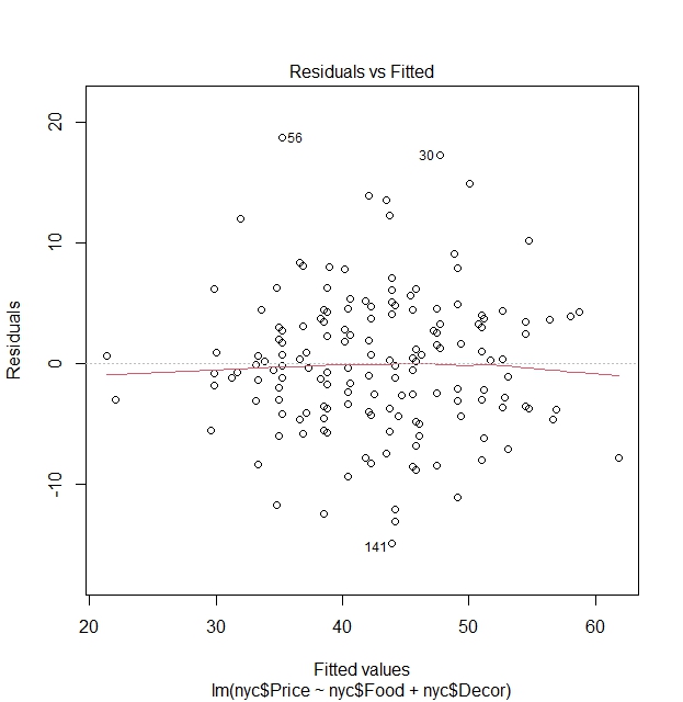
Residuals vs Fitted Values plot:
The aim of this of well-known plot is used to detect patterns and non-linearity of the model to help in addressing heteroscedasticity.
It has a red line that is a smoothed line of the residuals. The more straight and closer to $y=0$ this red line is, indicates that linearity assumption is satisfied in the model and the fact that mean of residuals is $0$.
There is also a dashed line at the y-axis at $0$ to show whether residuals are randomly spread across fitted values. If there is no discernible pattern of the residuals, we can say that the residuals exhibit approximately the same spread (variance) from $0$, satisying linear regression assumptions. If there is a discernible pattern in the residuals from the line $y=0$, it indicates a non-constant spread (variance) of residuals.
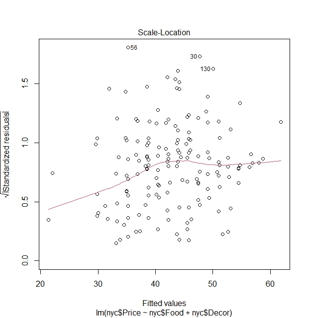
Scale-Location plot:
Plots squared root of absolute value of standardized residuals vs fitted values.
Why use standardized residuals? With standardized residuals that are independent of the scale of the response variable, we can compare such plots of different models easily without having to worry about the nature of the response variable.
Why the square root? It amplifies effect of residuals through giving a much more proportionate spread.
Why the absolute sign? It helps to only focus on the magnitude of residuals that can help visually because at times it can be hard to discern patterns when have positive or negative values.
It also has a red line that checks for linearity of residuals.
This graph has almost the similar function as the one above, but these modifications can in theory better help with the identification of heteroscedasticity when it is not quite obvious in the residuals vs fitted values plot.
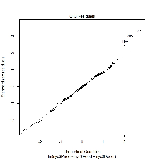
Quantile-Quantile (QQ) Plot of residuals:
This plots for normality of the residuals and aids us in finding out whether residuals satisfy assumption that it is normally distributed.
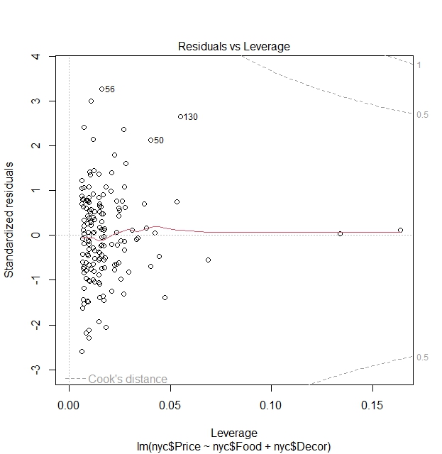
Residuals vs Leverage plot:
The purpose of this plot is to check for influential observations that can affect the model.
Leverage explains the extent to which coefficients in the regression model would change if an observation is removed.
The Cook’s distance line is a threshold (dashed-line) that decides whether a point is significantly influential. If a point is highly influential but does not lie inside the line, then it is concluded not to be influential.
If there is indeed such an influential observation, we should check for whether the observation is an error, or whether the influential observation stems from being estimated using a potentially wrong model.
Determine fit of model
By means of testing
Assume that we have $n$ observations, a $\text{Full}$ model that has $p_1 + p_2 = p$ parameters and a $\text{Part}$ model that has $p_2$ parameters which we write down it’s sum of squared residuals as $RSS_{full}$ and $RSS_{part}$. We aim to find out whether including or excluding $p_2$ parameters will be a better fit for the model. We are therefore dealing with the hypothesis test of whether coefficients belonging to these parameters $\theta_2$ are significantly different than zero.
\[H_0 : \theta_2 = 0 \quad \text{vs} \quad H_a: \theta_2 \neq 0\]F-Test
The F-test is typically used when we want to determine the model fit by considering whether a set of parameters are significantly different from zero in the model and makes use the sum of squared residuals (RSS) for it’s test statistic.
Why use RSS? The RSS essentially consists of the squared of errors that is also known as the unexplained variance in the model. It is thus a suitable variable to use for this purpose where we aim to find out if adding variables can significantly change this unexplained variance. This can be attributed to model fit.
The F-statistic goes as follows:
\[\text{F-statistic} = \frac{\frac{\text{RSS}_{Full} - \text{RSS}_{Part}}{p_{2}}}{\frac{\text{RSS}_{Part}}{n - p}} \sim F_{(p_{2}, n-p)}\]The essence of this test finds out whether difference between sum of squared residuals of models when $p_2$ is included and excluded of the different modelsare significant,. If it is, it serves as evidence that $p_2$ should be included.
Likelihood Ratio Test
This is an alternative to the F-test above.
Instead of using the log-likelihood, it is again replaced by the RSS. We should remember that the Likelihood Ratio Test is chi-squared distributed.
The chi-square test statistic is as follows:
\[2\mathcal{l}(\text{Full}) - 2\mathcal{l}(\text{Part}) = n \left( \log \text{RSS}_{Full} - \log \text{RSS}_{Part} \right) \sim \chi^2 (p_2)\]where the equality comes from the relationship between log-likelihood and RSS that is $\mathcal{l}(\theta) \approx -\frac{n}{2} \log(\text{RSS})$.
By means of cost values
Akaike Information Criterion
The AIC is a value that makes use of the number of parameters $p$ and log-likelihood $log(\mathcal{l})$ is formulated as follows:
\[\text{AIC} = - 2 \log(\mathcal{l}) + 2p\]It can be seen as a cost value for regression model selection. Hence the rule of thumb that we have to choose models with the lowest AIC or the lowest cost.
However, we have to note that the single value of the AIC will not help much in deduction of the best fit model so the point here is not to find the lowest possible AIC.
The essence rather lies on the relative differences between AIC’s of different models $\Delta \text{AIC} = \text{AIC}_1 - \text{AIC}_2$. If the difference is higher, it can tells us the cost is significantly reduced. This can be a basis to conclude that as the “cost” of your model becomes lower the more suitable the model is.
Bayesian Information Criterion
This is a variation of the AIC. The formula for BIC is as follows:
\[\text{BIC} = -2 \log L(\hat{\theta}) + p \log n\]The idea of remains the same as the AIC. We also should not take conclusions from a single value of the BIC but rather inspect the differences between BIC of models as well.
Remarks on AIC and BIC
Looking at the formula, we can see that adding more parameters $p$ add to the cost of the model, hence when it comes these values we aim to find the balance between model complexity and cost. We want to include more models that can help in explanation of the response variable, but we have to be aware that it comes at a cost.
Due to the $log(n)$ in the BIC formula, we should note that when $n \geq 8$ tells us that $log(n) \geq 2$. This means if when we estimate BIC of regression models (which will likely require way more than 8 observations), the part “$p\log n$” will greatly penalize the inclusion of more parameters compared to AIC. Hence, AIC is better suited for predictions (involving complex models) while BIC is better suited for simpler models.
Applying concepts to find best model fit in R using Sheather (2009) dataset
Knowing all the possible theories for model selection, we can now try to apply them in R. There are multiple methods in R on how we will be able to arrive at the best fit model.
In this, we aim to build a model that can explain Prices of a dinner in different Italian restaurants in New York City. The Price is therefore the response variable here.
The predictor variables which we can use are ratings of the “Food”, “Decoration” and “Service” (from 0 to 30) and the dummy variable “East” that tells us whether the location of the Italian restaurant is to the East or West of 5th Avenue.
Explanation on causality front of the dataset
Before we start, let us check on the causality of these variables to Price.
- There can be logical relationship between “Food”, “Decoration” and “Service” on “Price”. Good ratings of “Food”, “Service”, or “Decoration” individually or combined may potentially make restaurants charge more for the Price of dining in as demand for spots can become high due to these good characteristics of the restaurant.
- The inclusion of the “East” variable also has a logical explanation behind it. The 5th Avenue is seen as a dividing line between east and west of New York City in terms of demographics as the Upper East Side is known to be area that houses wealthy people and the high end shops are where tourists are rampant. Combination of these factors do indeed show that the variable “East” can affect price as restaurants lying on the east might charge more for wealthy people and tourists that may visit.
A conclusion is therefore that all the variables above may have an effect on “Price”, and it is for us to find out which model fits best. Below, I will use couple of these concepts to find the best model fit and see whether they will end up at the same “best” model.
F-test by aov() or anova() function
These two models have slightly different functions, but both aim to check the model fit.
aov() function
The aov() function only accepts one regression formula input (one model). It attempts to show the significance of every variable in model by the analysis of variance. The analysis of variance shows a significance of a variable in the model via whether a variable (regression sum of squares) significantly affects variation in the response (total sum of squares). One can see this as similar to the t-test where check for significance of every variable in the model.
Let us start by building couple of regression models. Some random possible linear combinations of these dataset is as follows:
reg1 <- lm(nyc$Price ~ nyc$Food)

reg2 <- lm(nyc$Price ~ nyc$Food + nyc$Decor)

reg3 <- lm(nyc$Price ~ nyc$Food + nyc$Decor + nyc$East)

reg4 <- lm(nyc$Price ~ nyc$Food + nyc$Decor + nyc$East + nyc$Service)
We can use aov() to check for significance of variables in every model.
# We can use aov() for reg1, showing results using summary()

summary(aov(reg1))

             Df Sum Sq Mean Sq F value Pr(>F)
nyc$Food      1   5670    5670   107.6 <2e-16 ***
Residuals   166   8751      53
---
Signif. codes:  0 ‘***’ 0.001 ‘**’ 0.01 ‘*’ 0.05 ‘.’ 0.1 ‘ ’ 1

# The above tells us that the variable "Food" (ratings of Food) is significant in explaining the variation of "Price".

summary(aov(reg2))

             Df Sum Sq Mean Sq F value Pr(>F)
nyc$Food      1   5670    5670  169.26 <2e-16 ***
nyc$Decor     1   3224    3224   96.23 <2e-16 ***
Residuals   165   5528      34
---
Signif. codes:  0 ‘***’ 0.001 ‘**’ 0.01 ‘*’ 0.05 ‘.’ 0.1 ‘ ’ 1

# "Food" and "Decor" (ratings of Food and Decoration) is significant in explaining variation of "Price".

summary(aov(reg3))

             Df Sum Sq Mean Sq F value Pr(>F)
nyc$Food      1   5670    5670 173.283 <2e-16 ***
nyc$Decor     1   3224    3224  98.515 <2e-16 ***
nyc$East      1    161     161   4.921 0.0279 *
Residuals   164   5367      33
---
Signif. codes:  0 ‘***’ 0.001 ‘**’ 0.01 ‘*’ 0.05 ‘.’ 0.1 ‘ ’ 1

# "Food" and "Decor" remain extremely significant. "East" (location of restaurant in East or West) is significant, but not much as "Food" and "Decor".

summary(aov(reg4))

             Df Sum Sq Mean Sq F value Pr(>F)
nyc$Food      1   5670    5670 172.227 <2e-16 ***
nyc$Decor     1   3224    3224  97.914 <2e-16 ***
nyc$East      1    161     161   4.891 0.0284 *
nyc$Service   1      0       0   0.000 0.9945
Residuals   163   5367      33
---
Signif. codes:  0 ‘***’ 0.001 ‘**’ 0.01 ‘*’ 0.05 ‘.’ 0.1 ‘ ’ 1

# "Food", "Decor" and "East" remains unchanged in terms significance. However, "Service" is not significant in explaining variation of "Price".

# The reader may also check that the significance (level of significance: * , **, ***) from the results of aov() will be the same as the t-test results from summary() of the regression models. The results will be not pasted here.

summary(reg1)
summary(reg2)
summary(reg3)
summary(reg4)
In conclusion, by the aov() method, we found out the insignificance of the variable “Service” in explaining food while the other three variables “Food”, “Decor” and “East” are significant.
anova() function
The anova() function is more flexible. It still uses the analysis of variance, but we are able to directly compare between full and nested models. It aids us in deciding whether addition of extra variables is necessary for the model.
# We can for instance compare directly reg1 to reg4 (simplest to most complex model) and test whether additional variables are jointly significant to the model by F-test.

anova(reg1, reg4)

Analysis of Variance Table

Model 1: nyc$Price ~ nyc$Food
Model 2: nyc$Price ~ nyc$Food + nyc$Decor + nyc$East + nyc$Service
  Res.Df    RSS Df Sum of Sq      F    Pr(>F)
1    166 8751.2
2    163 5366.5  3    3384.7 34.268 < 2.2e-16 ***
---
Signif. codes:  0 ‘***’ 0.001 ‘**’ 0.01 ‘*’ 0.05 ‘.’ 0.1 ‘ ’ 1
Doing this F-test tests joint significance of additional variables “Decor”, “East” and “Service” between reg1 and reg4. The null hypothesis tells us that all three additional variables are jointly not significant in explaining “Price”. The alternative hypothesis tells us that at least one of the three variables above are significant in explaining “Price”. If the alternative will hold, we still have to ask the question of the three is significant? We do not know. Therefore in a simpler model such as this however, it would be wise to conduct a step by step check by anova() and check for significance of every additional variable.
# We first compare the 2 simplest models and check whether additional variable of "Food" will help explain variation of "Price".

# Pay attention to the change in RSS values.

# We create one more regression model, of only the intercept, that is lm(nyc$Price ~ 1)

# We aim to begin this step by step test by looking if addition of "Food" will be significant in modelling "Price"

anova(lm(nyc$Price ~ 1), reg1)

Analysis of Variance Table

Model 1: nyc$Price ~ 1
Model 2: nyc$Price ~ nyc$Food
  Res.Df     RSS Df Sum of Sq      F    Pr(>F)
1    167 14421.5
2    166  8751.2  1    5670.3 107.56 < 2.2e-16 ***
---
Signif. codes:  0 ‘***’ 0.001 ‘**’ 0.01 ‘*’ 0.05 ‘.’ 0.1 ‘ ’ 1

# "Food" is confirmed to be an significant variable in explaining variation of "Price". We choose Model 2.

anova(reg1, reg2)

Analysis of Variance Table

Model 1: nyc$Price ~ nyc$Food
Model 2: nyc$Price ~ nyc$Food + nyc$Decor
  Res.Df    RSS Df Sum of Sq      F    Pr(>F)
1    166 8751.2
2    165 5527.5  1    3223.7 96.228 < 2.2e-16 ***
---
Signif. codes:  0 ‘***’ 0.001 ‘**’ 0.01 ‘*’ 0.05 ‘.’ 0.1 ‘ ’ 1

# "Decor" is significant variable in explaining variation of "Price". Model 2 chosen.

anova(reg2, reg3)

Analysis of Variance Table

Model 1: nyc$Price ~ nyc$Food + nyc$Decor
Model 2: nyc$Price ~ nyc$Food + nyc$Decor + nyc$Service
  Res.Df    RSS Df Sum of Sq      F Pr(>F)
1    165 5527.5
2    164 5523.6  1    3.9239 0.1165 0.7333

# "Service" is not significant in explaining variation in "Price". Model 1 chosen here.

# This would mean we should now compare $lm(nyc$Price ~ nyc$Food + nyc$Decor)$ with $lm(nyc$Price ~ nyc$Food + nyc$Decor + nyc$East)$

anova(reg2, lm(nyc$Price ~ nyc$Food + nyc$Decor + nyc$East))

Analysis of Variance Table

Model 1: nyc$Price ~ nyc$Food + nyc$Decor
Model 2: nyc$Price ~ nyc$Food + nyc$Decor + nyc$East
  Res.Df    RSS Df Sum of Sq      F  Pr(>F)
1    165 5527.5
2    164 5366.5  1    161.02 4.9207 0.02791 *
---
Signif. codes:  0 ‘***’ 0.001 ‘**’ 0.01 ‘*’ 0.05 ‘.’ 0.1 ‘ ’ 1

# We see "East" is still significant (though less strong than "Food" and "Decor") in explaining "Price". We choose Model 2 instead.
In conclusion, same as aov(), anova() tells us that “Food”, “Decor” and “East” explains the response “Price”.
Note that in more complex models, the step by step check as above would be too much work to do and is not necessary. The purpose of this anova() function is to compare models. In more complex models, this can be more of straightforward approach to directly build a model of best fit. What matters in the more complex model is the fact that we are able to find the best model that can potentially explain variation of the response. We do not have to know which of the X number of variables that are significant when the alternative hypothesis holds and this can be accounted for later in the analysis.
Backward Elimination: drop1() command in R
In backward elimination, we would often start with the full model, and the drop1() function will aid us in selecting the model that fits best by considering single term variable deletions from the full model. The test which we can use can be changed in the input of “test” as “F” (F-test) or “chisq” (chi-squared test).
drop1(reg4, test="F")

Single term deletions

Model:
nyc$Price ~ nyc$Food + nyc$Decor + nyc$Service + nyc$East
            Df Sum of Sq    RSS    AIC F value    Pr(>F)
<none>                   5366.5 591.95
nyc$Food     1     572.2 5938.7 606.97 17.3797 4.958e-05 ***
nyc$Decor    1    2550.8 7917.3 655.28 77.4763 1.869e-15 ***
nyc$Service  1       0.0 5366.5 589.95  0.0000   0.99452
nyc$East     1     157.1 5523.6 594.79  4.7716   0.03036 *
---
Signif. codes:  0 ‘***’ 0.001 ‘**’ 0.01 ‘*’ 0.05 ‘.’ 0.1 ‘ ’ 1
In every line, we test for between the model with the variable deletion every row and the full model $\text{lm(Price ~ Food + Decor + Service + East)}$ Below I interpret the results above:
In the row of nyc$Food:
- We test for the $H_0$: “Food” has no effect on model $\text{lm(Price ~ Decor + Service + East)}$ given presence of other predictors against $H_a$: “Food” has effect on model given presence of other predictors (full model).
- Low p-value of the F-statistic indicates we reject $H_0$ (part model) in favour of the $H_a$ that is the full model.
In the row of nyc$Decor:
- We test for the $H_0$: “Decor” has no effect on model $\text{lm(Price ~ Food + Service + East)}$ given presence of other predictors against $H_a$: “Decor” has effect on model given presence of other predictors (full model).
- Low p-value of the F-statistic indicates we reject $H_0$ (part model) in favour of the $H_a$ that is the full model.
In the row of nyc$Service:
- We test for the $H_0$: “Service” has no effect on model $\text{lm(Price ~ Food + Decor + East)}$ given presence of other predictors against $H_a$: “Service” has effect on model given presence of other predictors (full model).
- High p-value indicates that we do not reject $H_0$ (part model) in favour of the $H_a$ that is the full model.
In the row of nyc$East:
- We test for the $H_0$: “East” has no effect on model \text{lm(Price ~ Food + Decor + Service)} given presence of other predictors against $H_a$: “East” has effect on model given presence of other predictors (full model).
- Low p-value of the F-statistic indicates we reject $H_0$ (part model) in favour of the $H_a$ that is the full model.
To conclude, we see that in 3 of the 4 cases that we opt for the full model, but when we test for the exclusion of “Service”, we do indeed see evidence for the exclusion of nyc$Service instead of opting for the full model. This gives us evidence that we should pick the model of $\text{lm(Price ~ Food + Decor + East)}$.
To check whether we should still stick to this model, we conduct another backwards elimination test to check for certain if we can still drop other variables.
drop1(lm(nyc$Price ~ nyc$Food + nyc$Decor + nyc$East), test="F")

Single term deletions

Model:
nyc$Price ~ nyc$Food + nyc$Decor + nyc$East
          Df Sum of Sq    RSS    AIC  F value    Pr(>F)
<none>                 5366.5 589.95
nyc$Food   1    1115.2 6481.7 619.67  34.0788 2.759e-08 ***
nyc$Decor  1    3304.1 8670.6 668.55 100.9726 < 2.2e-16 ***
nyc$East   1     161.0 5527.5 592.91   4.9207   0.02791 *
---
Signif. codes:  0 ‘***’ 0.001 ‘**’ 0.01 ‘*’ 0.05 ‘.’ 0.1 ‘ ’ 1
We still see that low p-value of all three variables tested for exclusion rejects the null hypothesis of exclusion of the given variable. Hence, there is no variables that should be excluded through the test above, hence we stick to the model $\text{lm(Price ~ Food + Decor + East)}$.
To conclude, via the backwards elimination method, the model we choose therefore shows that “Food”, “Decor” and “East” are significant for explaining “Price”, but “Service” isn’t.
Forward Selection: add1() command in R
The forward selection method is simply the opposite of the backwards elimination method. Similar to how we conducted a step by step anova() analysis for model fit, we aim to add relevant variables one by one until we build the best model that contains significant predictors which can explain the variation of the response.
We start with simply the intercept, and see which one of the variables “Food”, “Decor”, “Service” or “East” is the best fit to add the model. The new model is then subjected to the same command add1() to add a new variable to further build to model. This goes on until the best fit model is found using all variables.
# The scope input in add1() is a term that specifies the terms to be considered for adding.

add1(reg0, test="F", scope=.~.+ nyc$Food + nyc$Decor + nyc$Service + nyc$East)

Single term additions

Model:
nyc$Price ~ 1
            Df Sum of Sq     RSS    AIC  F value  Pr(>F)
<none>                   14421.5 750.02
nyc$Food     1    5670.3  8751.2 668.10 107.5588 < 2e-16 ***
nyc$Decor    1    7566.8  6854.7 627.07 183.2432 < 2e-16 ***
nyc$Service  1    5928.1  8493.4 663.08 115.8627 < 2e-16 ***
nyc$East     1     502.3 13919.2 746.07   5.9906 0.01542 *
---
Signif. codes:  0 ‘***’ 0.001 ‘**’ 0.01 ‘*’ 0.05 ‘.’ 0.1 ‘ ’ 1
In this output, we test $H_0$ that is the inputted model of only the intercept $\text{lm(Price ~ 1)}$ against $H_a$ that is the single term addition models.
In the row nyc$Food:
- We test $H_0$ that is $\text{lm(Price ~ 1)}$ and $H_a$ that is $\text{lm(Price ~ Food)}$
- A low p-value tells us “Food” is significant, thus we should choose $H_a$, that is the model $\text{lm(Price ~ Food)}$.
In the row nyc$Decor:
- We test $H_0$ that is $\text{lm(Price ~ 1)}$ and $H_a$ that is $\text{lm(Price ~ Decor)}$
- A low p-value tells us “Decor” is significant, thus we should choose $H_a$, that is the model $\text{lm(Price ~ Decor)}$.
In the row nyc$Service:
- We test $H_0$ that is $\text{lm(Price ~ 1)}$ and $H_a$ that is $\text{lm(Price ~ Service)}$
- A low p-value tells us “Service” is significant, thus we should choose $H_a$, that is the model $\text{lm(Price ~ Service)}$.
In the row nyc$East:
- We test $H_0$ that is $\text{lm(Price ~ 1)}$ and $H_a$ that is $\text{lm(Price ~ East)}$
- A low p-value tells us “East” is significant, thus we should choose $H_a$, that is the model $\text{lm(Price ~ East)}$.
We see that all single addition models are significant. So how do we proceed in case of a tiebreaker such as this?
We use the AIC as a tiebreaker. We proceed with the model that has the lowest AIC, or the lowest cost.
Hence, we choose “Decor” $\text{lm(Price ~ Decor)}$, that happens to be the model that gives the lowest AIC of 627.07.
I will update the model reg0 by adding “Decor” using the command update().
reg0_update <- update(reg0, .~. + nyc$Decor)
We continue to find new single additions.
add1(reg0_update, test="F", scope=.~.+ nyc$Food + nyc$Service + nyc$East)

Single term additions

Model:
nyc$Price ~ nyc$Decor
            Df Sum of Sq    RSS    AIC F value    Pr(>F)
<none>                   6854.7 627.07
nyc$Food     1   1327.20 5527.5 592.91  39.618 2.682e-09 ***
nyc$Service  1    745.59 6109.2 609.72  20.137 1.347e-05 ***
nyc$East     1    373.07 6481.7 619.67   9.497  0.002412 **
---
Signif. codes:  0 ‘***’ 0.001 ‘**’ 0.01 ‘*’ 0.05 ‘.’ 0.1 ‘ ’ 1
In this new add1() test, we test the null hypothesis $H_0$: $\text{lm(Price ~ Decor)}$ on $H_a$ that is the single term additional models building up on $H_0$. I will not elaborate further on the structure of the $H_0$ and $H_a$. Reader can try to understand what every row tests for based on the explanation of the first add1() output above.
We see that “Food”, “Service” and “East” are the contenders for the next variable addition due to it’s significance, but the tiebreaker is broken by lower AIC value of “Food” that is $\text{lm(Price ~ Decor + Food)}$. Update the regression model as below by adding “Food”.
reg0_update_1 <- update(reg0_update, .~. + nyc$Food)
Onto the next single term addition
add1(reg0_update_1, test= "F", scope=.~. + nyc$Food + nyc$Decor + nyc$Service + nyc$East)

Single term additions

Model:
nyc$Price ~ nyc$Decor + nyc$Food
            Df Sum of Sq    RSS    AIC F value  Pr(>F)
<none>                   5527.5 592.91
nyc$Service  1     3.924 5523.6 594.79  0.1165 0.73330
nyc$East     1   161.019 5366.5 589.95  4.9207 0.02791 *
---
Signif. codes:  0 ‘***’ 0.001 ‘**’ 0.01 ‘*’ 0.05 ‘.’ 0.1 ‘ ’ 1
We see that “East” is the most significant variable to add to the model, based on p-value and also the AIC. We add “East” to the model.
reg0_update_2 <- update(reg0_update_1, .~.+ nyc$East)
Moving on to the last addition term:
add1(reg0_update_2, test="F", scope=.~. + nyc$Food + nyc$Decor + nyc$Service + nyc$East)

Single term additions

Model:
nyc$Price ~ nyc$Decor + nyc$Food + nyc$East
            Df Sum of Sq    RSS    AIC F value Pr(>F)
<none>                   5366.5 589.95
nyc$Service  1   0.00156 5366.5 591.95       0 0.9945
The final command checks if “Service” can be added to the model. By p-value, it is not significant at all. As a result, we stop at this model.
The best fit model by this add1() or forward selection is $\text{lm(Price ~ Decor + Food + East)}$.
The result is remarkably the same to the previous three where we showed that “Service” does not play a role in explaning “Price”.
$R^2$ (R-squared) Criteria
The R-squared criteria uses $R^2$ criteria to rank linear combinations of the “nyc” dataset based on it’s $R^2$ value. It makes use of the leaps() function.
library(leaps)

# The "int" input considers adding intercept for the model when conducting the exhaustive search

# As usual, the y (reponse) is "Price" (nyc[,3]) and x (predictors) are "Food", "Decor", "Service" and "East" (nyc[,4:7]).

M <- leaps(x = nyc[,4:7], y= nyc[,3], int=TRUE, method="r2")

$which
      1     2     3     4
1 FALSE  TRUE FALSE FALSE
1 FALSE FALSE  TRUE FALSE
1  TRUE FALSE FALSE FALSE
1 FALSE FALSE FALSE  TRUE
2  TRUE  TRUE FALSE FALSE
2 FALSE  TRUE  TRUE FALSE
2 FALSE  TRUE FALSE  TRUE
2  TRUE FALSE  TRUE FALSE
2 FALSE FALSE  TRUE  TRUE
2  TRUE FALSE FALSE  TRUE
3  TRUE  TRUE FALSE  TRUE
3  TRUE  TRUE  TRUE FALSE
3 FALSE  TRUE  TRUE  TRUE
3  TRUE FALSE  TRUE  TRUE
4  TRUE  TRUE  TRUE  TRUE

$label
[1] "(Intercept)" "1"           "2"           "3"           "4"

$size
 [1] 2 2 2 2 3 3 3 3 3 3 4 4 4 4 5

$r2
 [1] 0.52468652 0.41106077 0.39318352 0.03483085 0.61671564 0.57638643 0.55055537 0.44859379 0.41395090
[10] 0.39877199 0.62788083 0.61698772 0.58820412 0.45100737 0.62788094

# This gives a list of every possible linear combination and it's respective R-squared.
# TRUE/FALSE changed to 1/0 by cbind() function

cbind(M$which[order(M$r2), ], sort(M$r2))

  1 2 3 4
1 0 0 0 1 0.03483085
1 1 0 0 0 0.39318352
2 1 0 0 1 0.39877199
1 0 0 1 0 0.41106077
2 0 0 1 1 0.41395090
2 1 0 1 0 0.44859379
3 1 0 1 1 0.45100737
1 0 1 0 0 0.52468652
2 0 1 0 1 0.55055537
2 0 1 1 0 0.57638643
3 0 1 1 1 0.58820412
2 1 1 0 0 0.61671564
3 1 1 1 0 0.61698772
3 1 1 0 1 0.62788083
4 1 1 1 1 0.62788094

# 1st column tells us the number of variables in the model. Every row in the 2nd-5th column returns 1/0 that shows model of every possible combination of variables. The last column tells us the R-squared of every model combination from lowest to highest.
By this R-squared criteria, we see that the last 2 rows that is $\text{lm(Price ~ Food + Decor + East)}$ and $\text{lm(Price ~ Food + Decor + Service + East)}$ are fairly close in terms of the R-squared, with 0.62788083 and 0.62788094 respectively. Nevertheless, objectively using the rule of thumb of choosing the highest R-squared, we choose for the latter model instead.
AIC Forward Selection or Backward Elimination
We use the stepAIC() command as follows. It can use backward elimination and forward selection to choose models based on the lowest AIC value.
Let us first check this AIC method of Backward Elimination
# In backward elimination, we start with the full model, named reg4 we defined earlier.

stepAIC(reg4, scope=.~. + nyc$Food + nyc$Decor + nyc$Service + nyc$East, direction="backward")

Start:  AIC=591.95
nyc$Price ~ nyc$Food + nyc$Decor + nyc$Service + nyc$East

              Df Sum of Sq    RSS    AIC
- nyc$Service  1       0.0 5366.5 589.95
<none>                     5366.5 591.95
- nyc$East     1     157.1 5523.6 594.79
- nyc$Food     1     572.2 5938.7 606.97
- nyc$Decor    1    2550.8 7917.3 655.28

Step:  AIC=589.95
nyc$Price ~ nyc$Food + nyc$Decor + nyc$East

            Df Sum of Sq    RSS    AIC
<none>                   5366.5 589.95
- nyc$East   1     161.0 5527.5 592.91
- nyc$Food   1    1115.2 6481.7 619.67
- nyc$Decor  1    3304.1 8670.6 668.55

Call:
lm(formula = nyc$Price ~ nyc$Food + nyc$Decor + nyc$East)

Coefficients:
(Intercept)     nyc$Food    nyc$Decor     nyc$East
    -24.027        1.536        1.909        2.067
We see that removal of the “Service” gives the lowest AIC, hence in the first step it is removed. In the second step, we see that no removal of variables gives the lowest AIC, hence resulting in the best model (by means of AIC selection) of $\text{lm(Price ~ Food + Decor + East)}$.
# Now let us try forward selection using the AIC criterion. We start with the simplest model of only the intercept, stored as reg0 earlier.

stepAIC(reg0, scope=.~. + nyc$Food + nyc$Decor + nyc$Service + nyc$East, direction="forward")

Start:  AIC=750.02
nyc$Price ~ 1

              Df Sum of Sq     RSS    AIC
+ nyc$Decor    1    7566.8  6854.7 627.07
+ nyc$Service  1    5928.1  8493.4 663.08
+ nyc$Food     1    5670.3  8751.2 668.10
+ nyc$East     1     502.3 13919.2 746.07
<none>                     14421.5 750.02

Step:  AIC=627.07
nyc$Price ~ nyc$Decor

              Df Sum of Sq    RSS    AIC
+ nyc$Food     1   1327.20 5527.5 592.91
+ nyc$Service  1    745.59 6109.2 609.72
+ nyc$East     1    373.07 6481.7 619.67
<none>                     6854.7 627.07

Step:  AIC=592.91
nyc$Price ~ nyc$Decor + nyc$Food

              Df Sum of Sq    RSS    AIC
+ nyc$East     1   161.019 5366.5 589.95
<none>                     5527.5 592.91
+ nyc$Service  1     3.924 5523.6 594.79

Step:  AIC=589.95
nyc$Price ~ nyc$Decor + nyc$Food + nyc$East

              Df Sum of Sq    RSS    AIC
<none>                     5366.5 589.95
+ nyc$Service  1   0.00156 5366.5 591.95

Call:
lm(formula = nyc$Price ~ nyc$Decor + nyc$Food + nyc$East)

Coefficients:
(Intercept)    nyc$Decor     nyc$Food     nyc$East
    -24.027        1.909        1.536        2.067
We see that this AIC forward selection first adds “Decor”, then “Food”, and lastly “East”. In the last part of the output, adding nothing gives a more lower AIC compared to adding “Service” hence we do not add “Service” based on the low AIC criteria. Hence, same as the AIC backward elimination, AIC forward selection yields the best fit model (based on AIC criteria) of $\text{lm(Price ~ Food + Decor + East)}$.
The final model to choose: remarks
Based on the different model selection methods above, I summarize the best fit model from different methods.
aov():
$\text{lm(Price ~ Food + Decor + East)}$
anova():
$\text{lm(Price ~ Food + Decor + East)}$
drop1():
$\text{lm(Price ~ Food + Decor + East)}$
add1():
$\text{lm(Price ~ Food + Decor + East)}$
leaps():
$\text{lm(Price ~ Food + Decor + East + Service)}$
stepAIC():
-
Forward Selection: $\text{lm(Price ~ Food + Decor + East)}$
-
Backward Elimination: $\text{lm(Price ~ Food + Decor + East)}$
Of course in one’s own research, doing all of the selection processes above is not necessary. What methods to be used depends on the context of research. We should also be aware that different methods may produce different best fit models as shown above.
Based on the above, I decide to choose $\text{lm(Price ~ Food + Decor + East)}$ as the best fit model.
This based on how majority of selection methods converged on this model, how it contains all significant variables that explain the response “Price”, the R-squared, which we remember was almost close to the highest R-squared from the possible linear combinations shown in the leaps() command.
Interpreting the chosen best fit model
Let us try to interpret the output of the best fit regression model.
summary(lm(nyc$Price~nyc$Food+nyc$Decor+nyc$East))

Call:
lm(formula = nyc$Price ~ nyc$Food + nyc$Decor + nyc$East)

Residuals:
     Min       1Q   Median       3Q      Max
-14.0451  -3.8809   0.0389   3.3918  17.7557

Coefficients:
            Estimate Std. Error t value Pr(>|t|)
(Intercept) -24.0269     4.6727  -5.142 7.67e-07 ***
nyc$Food      1.5363     0.2632   5.838 2.76e-08 ***
nyc$Decor     1.9094     0.1900  10.049  < 2e-16 ***
nyc$East      2.0670     0.9318   2.218   0.0279 *
---
Signif. codes:  0 ‘***’ 0.001 ‘**’ 0.01 ‘*’ 0.05 ‘.’ 0.1 ‘ ’ 1

Residual standard error: 5.72 on 164 degrees of freedom
Multiple R-squared:  0.6279,	Adjusted R-squared:  0.6211
F-statistic: 92.24 on 3 and 164 DF,  p-value: < 2.2e-16
Intercept (Baseline Value of Price):
Assuming that all attributes (predictors) are 0, meaning if a restaurant lies on the East of 5th avenue, and has the lowest possible ratings that is $0$ for Food, Decor then the Italian restaurant would be losing $24.0269$ on average, which directionally makes sense based on the causal theories. Low ratings mean less visitors and restaurant makes a loss. Additionally, being on the east of 5th avenue, where there can be fewer people visiting, than on the west of 5th avenue adds up to the directional bias we see in this intercept.
“Food” to “Price”:
This tells us that if food ratings go up by 1 point, the average price of a dinner in a Italian restaurant will go up by $1.5363. Coefficient agrees with causality theory.
“Decor” to “Price”:
This tells us that if decoration ratings go up by 1 point, the average price of a dinner in a Italian restaurant will go up by $1.9094. Coefficient agrees with causality theory
“East” to “Price”:
This is a dummy variable. How we interpret this is that Italian restaurants in the east of 5th Avenue charge on average $2.0670 more than Italian restaurants in the west of 5th Avenue. Coefficient agrees with causality theory.
Checking whether regression assumptions hold
Let us check the first two plots of the plot() of the regression model.
Homoscedasticity
plot(lm(nyc$Price~nyc$Food+nyc$Decor+nyc$East))
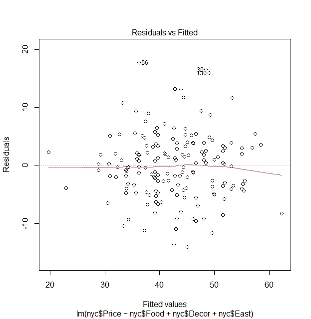
We see via the residuals vs fitted value graph that there is no clear pattern between residuals and fitted values and that points vary around the line of $\text{Residuals}=0$, hence a clear indication that variances of residuals are constant an that homoscedasticity holds.
Normality of errors
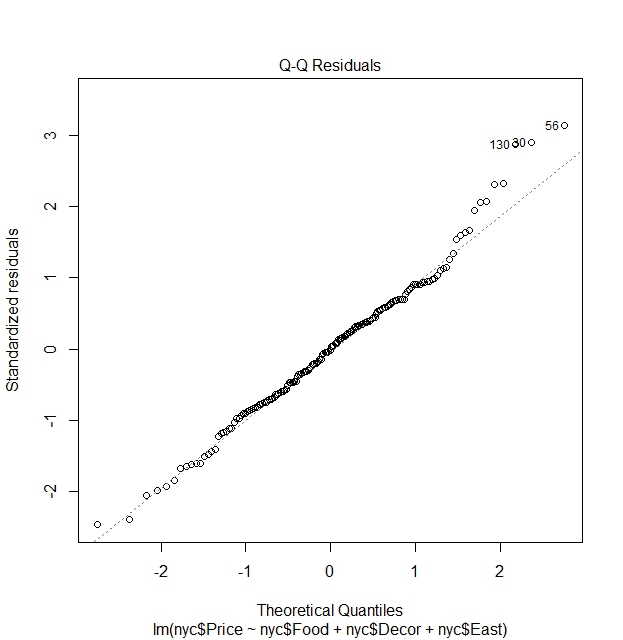
We see that the residuals are fairly normally distributed, except for some outlier points that strays from normality. These are the outlier points in the dataset
nyc[130,]

nyc[30,]

nyc[56,]

    Case    Restaurant Price Food Decor Service East
130  130 Rainbow Grill    65   19    23      18    0
   Case     Restaurant Price Food Decor Service East
30   30 Harry Cipriani    65   21    20      20    1
   Case Restaurant Price Food Decor Service East
56   56      Nello    54   18    16      15    1
What we can learn here is indeed see that there are outlier points where ratings are not proportionate to the price. In this case, despite low ratings, restaurants still charge high prices.
We do not expect perfect normality from the residuals. We often see it as sufficient to simply report the presence of such outliers during our analysis.
Investigating why “Service” is not significant in the full model
In terms of causality as I elaborated, the full model of $\text{lm(Price ~ Food + Decor + Service + East)}$ would make more sense causality-wise. However, a slight problem in the model as one might have caught on is the insignificance of “Service” itself when combined with other variables.
Could this mean the full model is not that accurate after all and that a new model is needed?
Let us first look at the pairwise plots to check the pairwise relationships between response variable “Price” and the possible predictor variables “Food”, “Decor”, “Service” and “East”.
pair.panels(nyc[,3:7])
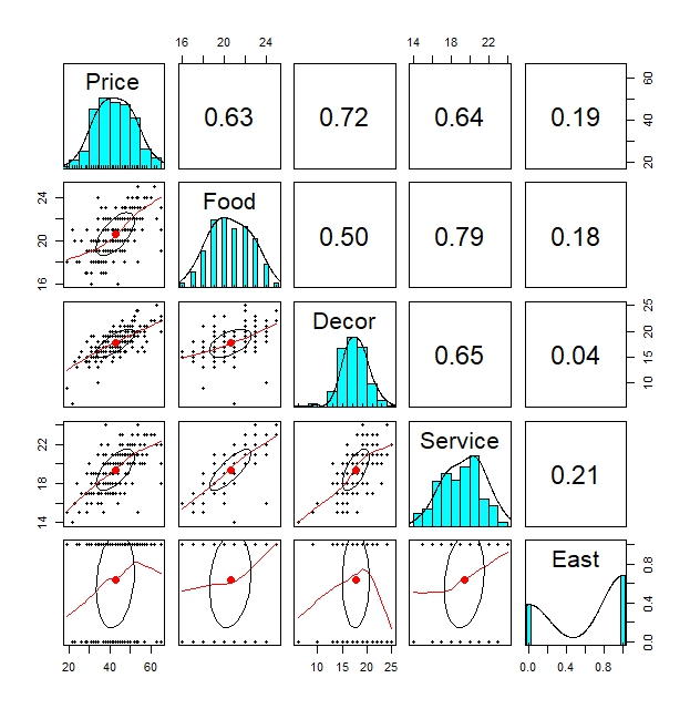
By this pairwise plots, we clearly see a moderately high correlation between “Service” and “Food” of around 0.64
Note that we did not catch this effect due to the fact we built our initial random models as starting from $\text{lm(Price~Food)}$. Remember objects reg0 - reg4.
We can confirm this relationship further by regressing “Price” on “Service”, which shows “Service” clearly has an significant effect on “Price”.
summary(lm(nyc$Price ~ nyc$Service))

Call:
lm(formula = nyc$Price ~ nyc$Service)

Residuals:
     Min       1Q   Median       3Q      Max
-17.6646  -4.7540  -0.2093   4.3368  26.2460

Coefficients:
            Estimate Std. Error t value Pr(>|t|)
(Intercept) -11.9778     5.1093  -2.344   0.0202 *
nyc$Service   2.8184     0.2618  10.764   <2e-16 ***
---
Signif. codes:  0 ‘***’ 0.001 ‘**’ 0.01 ‘*’ 0.05 ‘.’ 0.1 ‘ ’ 1

Residual standard error: 7.153 on 166 degrees of freedom
Multiple R-squared:  0.4111,	Adjusted R-squared:  0.4075
F-statistic: 115.9 on 1 and 166 DF,  p-value: < 2.2e-16
Conducting further regressions, I also found that “Service” remained significant when we added a second variable “Food”, “Decor” or “East”.
summary(lm(nyc$Price~nyc$Service+nyc$Decor))

Call:
lm(formula = nyc$Price ~ nyc$Service + nyc$Decor)

Residuals:
     Min       1Q   Median       3Q      Max
-13.7411  -3.7754  -0.8103   4.0936  20.1530

Coefficients:
            Estimate Std. Error t value Pr(>|t|)
(Intercept) -15.0615     4.3633  -3.452 0.000707 ***
nyc$Service   1.3085     0.2916   4.487 1.35e-05 ***
nyc$Decor     1.8301     0.2281   8.025 1.80e-13 ***
---
Signif. codes:  0 ‘***’ 0.001 ‘**’ 0.01 ‘*’ 0.05 ‘.’ 0.1 ‘ ’ 1

Residual standard error: 6.085 on 165 degrees of freedom
Multiple R-squared:  0.5764,	Adjusted R-squared:  0.5713
F-statistic: 112.3 on 2 and 165 DF,  p-value: < 2.2e-16

summary(lm(nyc$Price~nyc$Service+nyc$Food))

Call:
lm(formula = nyc$Price ~ nyc$Service + nyc$Food)

Residuals:
     Min       1Q   Median       3Q      Max
-16.1333  -4.7053   0.4169   3.5992  27.0728

Coefficients:
            Estimate Std. Error t value Pr(>|t|)
(Intercept) -21.1586     5.6651  -3.735 0.000258 ***
nyc$Service   1.7041     0.4185   4.072 7.22e-05 ***
nyc$Food      1.4954     0.4462   3.351 0.000997 ***
---
Signif. codes:  0 ‘***’ 0.001 ‘**’ 0.01 ‘*’ 0.05 ‘.’ 0.1 ‘ ’ 1

Residual standard error: 6.942 on 165 degrees of freedom
Multiple R-squared:  0.4486,	Adjusted R-squared:  0.4419
F-statistic: 67.12 on 2 and 165 DF,  p-value: < 2.2e-16

summary(lm(nyc$Price~nyc$Service+nyc$East))

Call:
lm(formula = nyc$Price ~ nyc$Service + nyc$East)

Residuals:
     Min       1Q   Median       3Q      Max
-17.8216  -4.8080  -0.4821   4.7460  26.8413

Coefficients:
            Estimate Std. Error t value Pr(>|t|)
(Intercept) -11.6636     5.1240  -2.276   0.0241 *
nyc$Service   2.7679     0.2679  10.331   <2e-16 ***
nyc$East      1.0555     1.1702   0.902   0.3683
---
Signif. codes:  0 ‘***’ 0.001 ‘**’ 0.01 ‘*’ 0.05 ‘.’ 0.1 ‘ ’ 1

Residual standard error: 7.157 on 165 degrees of freedom
Multiple R-squared:  0.414,	Adjusted R-squared:  0.4068
F-statistic: 58.27 on 2 and 165 DF,  p-value: < 2.2e-16
However, when we start to add a third variable of either “Food” or “Decor”, making the model of $\text{lm(Price ~ Service + Decor + Food)}$, “Service” becomes insignificant.
In the other possible three-variable regression models of $\text{lm(Price ~ Service + Decor + East)}$ and $\text{lm(Price ~ Service + Food + East)}$, we see that “Service” does not become insignificant.
When we add a fourth variable, “Service” remains insignificant. These are shown below:
summary(lm(nyc$Price~nyc$Service+nyc$Decor+nyc$Food))

Call:
lm(formula = nyc$Price ~ nyc$Service + nyc$Decor + nyc$Food)

Residuals:
     Min       1Q   Median       3Q      Max
-14.8440  -3.7039  -0.1525   3.6218  19.0576

Coefficients:
            Estimate Std. Error t value Pr(>|t|)
(Intercept) -24.6409     4.7536  -5.184 6.33e-07 ***
nyc$Service   0.1350     0.3957   0.341    0.733
nyc$Decor     1.8473     0.2176   8.491 1.17e-14 ***
nyc$Food      1.5556     0.3731   4.170 4.93e-05 ***
---
Signif. codes:  0 ‘***’ 0.001 ‘**’ 0.01 ‘*’ 0.05 ‘.’ 0.1 ‘ ’ 1

Residual standard error: 5.803 on 164 degrees of freedom
Multiple R-squared:  0.617,	Adjusted R-squared:   0.61
F-statistic: 88.06 on 3 and 164 DF,  p-value: < 2.2e-16

summary(lm(nyc$Price~nyc$Service+nyc$Decor+nyc$East))

Call:
lm(formula = nyc$Price ~ nyc$Service + nyc$Decor + nyc$East)

Residuals:
    Min      1Q  Median      3Q     Max
-14.514  -3.668  -0.769   3.704  18.778

Coefficients:
            Estimate Std. Error t value Pr(>|t|)
(Intercept) -14.5308     4.3220  -3.362 0.000963 ***
nyc$Service   1.1513     0.2973   3.872 0.000156 ***
nyc$Decor     1.8956     0.2276   8.331 3.05e-14 ***
nyc$East      2.1535     0.9927   2.169 0.031489 *
---
Signif. codes:  0 ‘***’ 0.001 ‘**’ 0.01 ‘*’ 0.05 ‘.’ 0.1 ‘ ’ 1

Residual standard error: 6.018 on 164 degrees of freedom
Multiple R-squared:  0.5882,	Adjusted R-squared:  0.5807
F-statistic: 78.09 on 3 and 164 DF,  p-value: < 2.2e-16

summary(lm(nyc$Price~nyc$Service+nyc$Food+nyc$East))

Call:
lm(formula = nyc$Price ~ nyc$Service + nyc$Food + nyc$East)

Residuals:
     Min       1Q   Median       3Q      Max
-16.2862  -4.5254   0.3421   3.7079  27.6119

Coefficients:
            Estimate Std. Error t value Pr(>|t|)
(Intercept) -20.8155     5.6843  -3.662 0.000337 ***
nyc$Service   1.6647     0.4214   3.950 0.000116 ***
nyc$Food      1.4863     0.4467   3.327 0.001083 **
nyc$East      0.9649     1.1363   0.849 0.397053
---
Signif. codes:  0 ‘***’ 0.001 ‘**’ 0.01 ‘*’ 0.05 ‘.’ 0.1 ‘ ’ 1

Residual standard error: 6.948 on 164 degrees of freedom
Multiple R-squared:  0.451,	Adjusted R-squared:  0.441
F-statistic: 44.91 on 3 and 164 DF,  p-value: < 2.2e-16

summary(lm(nyc$Price~nyc$Service+nyc$Decor+nyc$East+nyc$Food))

Call:
lm(formula = nyc$Price ~ nyc$Service + nyc$Decor + nyc$East +
    nyc$Food)

Residuals:
     Min       1Q   Median       3Q      Max
-14.0465  -3.8837   0.0373   3.3942  17.7491

Coefficients:
              Estimate Std. Error t value Pr(>|t|)
(Intercept) -24.023800   4.708359  -5.102 9.24e-07 ***
nyc$Service  -0.002727   0.396232  -0.007   0.9945
nyc$Decor     1.910087   0.217005   8.802 1.87e-15 ***
nyc$East      2.068050   0.946739   2.184   0.0304 *
nyc$Food      1.538120   0.368951   4.169 4.96e-05 ***
---
Signif. codes:  0 ‘***’ 0.001 ‘**’ 0.01 ‘*’ 0.05 ‘.’ 0.1 ‘ ’ 1

Residual standard error: 5.738 on 163 degrees of freedom
Multiple R-squared:  0.6279,	Adjusted R-squared:  0.6187
F-statistic: 68.76 on 4 and 163 DF,  p-value: < 2.2e-16
We see that on the four models above that there is an overlap in explanatory power of “Food”, “Decor” and “Service”. As a result, in models where “Food” and “Decor” are present together alongside “Service”, “Service” becomes insignificant but in models where “Food” and “Decor” are not present together, “Service” remains significant. What we conclude from the above is that there is some kind of dependency between the three variables of “Food”, “Decor” and “Service”.
What can be logical explanation for these dependence? It can be said that better “Food” and “Decor” could go hand in hand with better “Service”. As a result, “Food” and “Decor” captured majority of the variation on “Price”, resulting in “Service” being insignificant.
There are a few solutions to this:
- Remove “Service” completely from the model because we aim to find the most complete model. It appears that “Service” does not explain much in the full model, and this is enough reason to drop it.
- We can try to add interaction terms, however it is often times not suggested as it may lead to complicating the model. We should try to only add interaction terms when we can support it by theory, which in this case, we can.
Model with Interaction Terms
Here, we try two models that use interaction terms between “Service” on “Food” or “Price”.
summary(lm(nyc$Price ~ nyc$Service:nyc$Decor + nyc$Food + nyc$East))

Call:
lm(formula = nyc$Price ~ nyc$Service:nyc$Decor + nyc$Food + nyc$East)

Residuals:
     Min       1Q   Median       3Q      Max
-15.1012  -3.5422  -0.0879   3.4140  20.5181

Coefficients:
                      Estimate Std. Error t value Pr(>|t|)
(Intercept)           0.452969   5.212134   0.087    0.931
nyc$Food              0.775154   0.332542   2.331    0.021 *
nyc$East              1.583350   0.968071   1.636    0.104
nyc$Service:nyc$Decor 0.072887   0.008123   8.973  6.4e-16 ***
---
Signif. codes:  0 ‘***’ 0.001 ‘**’ 0.01 ‘*’ 0.05 ‘.’ 0.1 ‘ ’ 1

Residual standard error: 5.955 on 164 degrees of freedom
Multiple R-squared:  0.5967,	Adjusted R-squared:  0.5894
F-statistic:  80.9 on 3 and 164 DF,  p-value: < 2.2e-16

summary(lm(nyc$Price ~ nyc$Service:nyc$Food + nyc$Decor + nyc$East))

Call:
lm(formula = nyc$Price ~ nyc$Service:nyc$Food + nyc$Decor + nyc$East)

Residuals:
     Min       1Q   Median       3Q      Max
-13.7735  -3.6537  -0.2284   3.7593  18.9379

Coefficients:
                      Estimate Std. Error t value Pr(>|t|)
(Intercept)          -5.863007   3.064891  -1.913   0.0575 .
nyc$Decor             1.763692   0.213458   8.262 4.57e-14 ***
nyc$East              1.856157   0.958367   1.937   0.0545 .
nyc$Service:nyc$Food  0.040185   0.007594   5.291 3.84e-07 ***
---
Signif. codes:  0 ‘***’ 0.001 ‘**’ 0.01 ‘*’ 0.05 ‘.’ 0.1 ‘ ’ 1

Residual standard error: 5.81 on 164 degrees of freedom
Multiple R-squared:  0.6161,	Adjusted R-squared:  0.6091
F-statistic: 87.73 on 3 and 164 DF,  p-value: < 2.2e-16
Using the interaction term “Decor” and “Service” is not appropriate as it made the model stray off from theory, especially looking at the intercept that is not significant anymore and also in the wrong sign. Not having a baseline value is a sign that tells us something in the model is wrong.
On the other hand, we see that interaction term of “Food” and “Service” is significant and can be appropriate as it produces a model whose intercept and coefficient signs still agree with theory and still significant in at least the 10% level. The positive sign of the interaction term coefficient tells us that the higher the rating of Food, the more positively stronger Service is to the Price. This agrees with theory that states good Service tends to come with good Food, which will increase Price.
Model with Interaction Term vs Best Fit Model: Which to choose?
Comparing the interaction model (“Service” and “Food”) to the best fit model we concluded earlier:
summary(lm(nyc$Price~nyc$Food+nyc$Decor+nyc$East))

Call:
lm(formula = nyc$Price ~ nyc$Food + nyc$Decor + nyc$East)

Residuals:
     Min       1Q   Median       3Q      Max
-14.0451  -3.8809   0.0389   3.3918  17.7557

Coefficients:
            Estimate Std. Error t value Pr(>|t|)
(Intercept) -24.0269     4.6727  -5.142 7.67e-07 ***
nyc$Food      1.5363     0.2632   5.838 2.76e-08 ***
nyc$Decor     1.9094     0.1900  10.049  < 2e-16 ***
nyc$East      2.0670     0.9318   2.218   0.0279 *
---
Signif. codes:  0 ‘***’ 0.001 ‘**’ 0.01 ‘*’ 0.05 ‘.’ 0.1 ‘ ’ 1

Residual standard error: 5.72 on 164 degrees of freedom
Multiple R-squared:  0.6279,	Adjusted R-squared:  0.6211
F-statistic: 92.24 on 3 and 164 DF,  p-value: < 2.2e-16
We still see that the best fit model above still has the edge over the model with interaction terms in terms of R-squared and how it has a lower spread of residuals.
So what model do we choose in the end?
- If we aim to find the best fit model that best explains the variation in Price, then we choose for the best fit model objectively based on factors such as R-squared and on which model minimizes most residuals.
- If the aim was to focus on why “Service” was not significant in the full model, we may emphasize on the possible interaction between “Service” and “Food” and/or “Service”. We showed earlier that the model with interaction “Service” and “Food” was able to explain the variation in price significantly while keeping other elements such as the intercept and other coefficients align in it’s directional bias of causality while at the same time retaining their respective significance. We may also argue that it’s R-squared is not far off from the best-fit model, hence concluding that with the interaction model we may get a better coverage of the variation of “Price” rather than sticking with the linear best fit model.
To sum it all up, which model we choose in the end, depends on the context of our research.
Conclusion
In this article, I went through the steps on what we should consider when doing regression. What models should we choose? How do we arrive at the best model and what factors should we consider? These are elementary questions that we will encounter when doing regression. I have given an example to tackle these questions using the Sheather (2009) dataset. I hope you have found this article helpful.
Dataset and R-Script Download
The R-Script, along with the dataset, can be downloaded from the assets directory in my GitHub repository. The R code is under the folder “codes”, named AppRegression_Rcode_Actuary492.R and the dataset lies under the folder “dataset”, named nyc.csv
References
McQuire, A., & Kume, M. (2020). R Programming for Actuarial Science. Wiley.
Leave a comment