Linear Regression

Regression lies at the heart of science. This concept is useful when we aim to investigate whether some predictor variable has an effect to some response variable and potentially quantify it’s effect. In risk management modelling, think for instance investigating whether age, location or number of claims in a previous period of the individual may have an effect on the claims in the current period. Having an overview of all possible factors that can influence claims is important to get an overview of where one’s risk is precisely coming from. In fact, this analysis does require a variation of the regression method than the one we will be discussing in this article. Here, I will only explain the basic concept of linear regression, and further articles shall follow on the different types of regression models.

Regression

The regression model theory is expressed as follows:

\[Y = f(X_1, X_2, ... , X_p) + error\]

where $f(\cdot)$ is essentially some objective function that can be linear, polynomial containing predictor variables $(X_1, … , X_p)$ that attempts to model or explain the response variable $Y$ and predict potential reponses $\hat{Y}$. In this article, we will be only focusing on linear regression, where the regression model shall only contain predictor variables of at most to the power of $1$.

Simple Linear Regression Model

The simple linear regression model attempts to find the effect of ONE predictor $x_i$ on the response $y_i$. We also have the case when multiple predictors are involved (multiple linear regression model) however in this section I am going to focus on the simple linear regression. Assume that we have a dataset of pairs $(x_i, y_i)$ from $i = 1,2,…, p$. We can express the supposedly linear relationship between $y_i$ and $x_i$ as follows:

\[y_i = \beta_0 + \beta_1 x_i + e_i\]

The $\alpha$ and $\beta$ are coefficients to be calculated in order to fit the model and to quantify the relationship between the predictor $x_i$ and response $y_i$. The error term $e_i$ is the difference between the observed $y_i$ and the estimated $\hat{y_i}$ using the estimated coefficients $\hat{\alpha}$ and $\hat{\beta}$ and the given fixed $x_i$ observations.

\[\hat{y_i} = \hat{\beta_0} + \hat{\beta_1} x_i\] \[e_i = y_i - \hat{y_i} = y_i - \hat{\beta_0} - \hat{\beta_1} x_i\]

Assumptions of the Simple Linear Regression Model

There are two important assumptions in this model:

• Errors in the model are not correlated in any way with each other
• Errors are i.i.d (independent and identically distributed) conditionally normally distributed $e_i \mid x_i$ with mean 0 and finite constant variance $\sigma^2$.

Why conditional on $X=x$? Fixed $x_i$’s are assumed in order to generate predictions $\hat{y_i}$ used to calculate errors. Random error realisations therefore require fixed $x_i$.

\[e_i|x_i \sim N(0, \sigma^2)\]

This means that the average of errors shall be zero meaning the model shall not over-or-underpredict $y_i$. The constant variance tells us that spread of errors must remain the same across all values of the predictor $x_i$. If the spread of errors is different for different fixed $x_i$, it tells us that the model predictions are reliable for some values of $x_i$ than the others, which can invalidate conclusions from the model.

As $y_i$ is directly dependent on the errors $e_i$ = $y_i$ - $\hat{y_i}$, it means that we need to know for this linear regression model is that the response $y_i$ must strictly be a continuous variable in order to satisfy the continuous nature of the normally-distributed errors and make sense of the linear regression model (remember normal distribution is a continuous distribution).

However, $x_i$ can be discrete or continuous because the model is conditional on $x_i$ being fixed. As long as one can show $y_i$ can vary through $x_i$, the model shall hold regardless whether $x_i$ is discrete or continuous.

With these assumptions in mind, we can also find the distribution of $y_i$ that we should directly follow the normal distribution through it’s errors:

\[E[y_i|x_i] = E[\beta_0 + \beta_1 x_i + e_i|x_i] = \beta_0 + \beta_1 x_i + E[e_i|x_i] = \beta_0 + \beta_1 x_i + 0 = \beta_0 + \beta_1 x_i\] \[Var[y_i|x_i] = Var[\beta_0 + \beta_1 x_i + e_i|x_i] = Var[e_i|x_i] = \sigma^2\] \[y_i|x_i \sim N(\beta_0 + \beta_1 x_i , \sigma^2)\]

Finding $\beta_0$ and $\beta_1$ through calculations

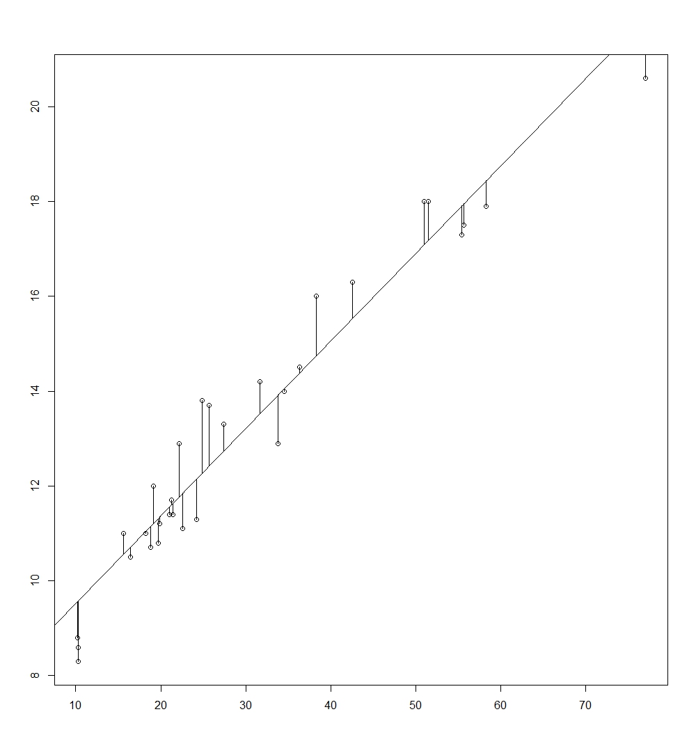
Finding $\beta_0$ and $\beta_1$ is done through the condition that these coefficients can arrive at a model that can minimize the sum of squared residual errors. We know that error is the difference between the observed response $y_i$ and the estimated response from the regression model $\hat{y_i}$.

\[\min_{\hat{\beta_0}, \hat{\beta_1}} \sum_{i=1}^{n} e_i^2 = \min_{\hat{\beta_0}, \hat{\beta_1}} \sum_{i=1}^{n} (y_i - \hat{y_i})^2\]

In other words, the $\beta_0$ and $\beta_1$ is calculated such that it produces the regression line (made out of paired observations of predicted $\hat{y_i}$ values and $x_i$) that minimizes the distance between the observations ($x_i$, $y_i$) to the regression line. Visualised, it looks as such:

The values of $\hat{\beta_0}$ and $\hat{\beta_1}$ is as follows.

\[\hat{\beta_0} = \bar{y_i} - \hat{\beta_1} \bar{x_i} \quad \hat{\beta_1} = \frac{cov(x_i,y_i)}{cov(x_i,x_i)}\]

Let me take you through how you can derive $\alpha$ and $\beta$.

\[\min_{\hat{\beta_0}, \hat{\beta_1}} \sum_{i=1}^{n} (y_i - \hat{y_i})^2 = \min_{\hat{\beta_0}, \hat{\beta_1}} \sum_{i=1}^{n} (y_i - \hat{\beta_0} - \hat{\beta_1} x_i)^2\]

Deriving $\hat{\beta_0}$ by minimization:

\[\frac{d}{d_\hat{\beta_0}} \sum_{i=1}^{n} (y_i - \hat{\beta_0} - \hat{\beta_1} x_i)^2 = 0\] \[\sum_{i=1}^{n} 2*(y_i - \hat{\beta_0} - \hat{\beta_1} x_i)*(-1) = 0 \rightarrow \sum_{i=1}^{n} (y_i - \hat{\beta_0} - \hat{\beta_1} x_i) = 0\]

We split the summation into own terms:

\[\sum_{i=1}^{n} y_i - \sum_{i=1}^{n} \hat{\beta_0} - \sum_{i=1}^{n} \hat{\beta_1} x_i = 0 \rightarrow \sum_{i=1}^{n} y_i - n\hat{\beta_0} - \hat{\beta_1} \sum_{i=1}^{n} x_i = 0\]

Using the relationship $\sum_{i=1}^{n} a_i = n*\frac{1}{n} \sum_{i=1}^{n} a_i = n \bar{a_i}$

\[n*\bar{y_i} - n\hat{\beta_0} - \beta n \bar{x_i} = 0 \rightarrow n*(\bar{y_i} - \hat{\beta_0} - \hat{\beta_1} \bar{x_i}) = 0 \rightarrow \bar{y_i} - \hat{\beta_0} - \hat{\beta_1} \bar{x_i} = 0\]

Moving $\hat{\beta_0}$ to other side we get the estimate:

\[\hat{\beta_0} = \bar{y_i} - \hat{\beta_1} \bar{x_i}\]

Now, deriving $\hat{\beta_1}$:

\[\frac{d}{d_\hat{\beta_1}} \sum_{i=1}^{n} (y_i - \hat{\beta_0} - \hat{\beta_1} x_i)^2 = 0\] \[\sum_{i=1}^{n} 2*(y_i - \hat{\beta_0} - \hat{\beta_1} x_i) * (-x_i) = 0 \rightarrow \sum_{i=1}^{n} (y_i - \hat{\beta_0} - \hat{\beta_1} x_i)*(x_i) = 0\]

Splitting summation in individual terms:

\[\sum_{i=1}^{n} y_i x_i - \sum_{i=1}^{n} \hat{\beta_0} x_i - \sum_{i=1}^{n} \hat{\beta_1} x_i x_i = 0 \rightarrow \sum_{i=1}^{n} y_i x_i - \hat{\beta_0} \sum_{i=1}^{n} x_i - \hat{\beta_1} \sum_{i=1}^{n} x_i = 0\]

Plugging in $\hat{\beta_0}$ into the last equation above:

\[\sum_{i=1}^{n} y_i x_i - (\bar{y_i} - \hat{\beta_1} \bar{x_i}) \sum_{i=1}^{n} x_i - \hat{\beta_1} \sum_{i=1}^{n} x_i = 0\]

Expanding equation further:

\[\sum_{i=1}^{n} y_i x_i - \bar{y_i} \sum_{i=1}^{n} x_i + \hat{\beta_1} \bar{x_i} \sum_{i=1}^{n} x_i - \hat{\beta_1} \sum_{i=1}^{n} x_i = 0\] \[\sum_{i=1}^{n} y_i x_i - \bar{y_i} \sum_{i=1}^{n} x_i - \hat{\beta_1}*(\sum_{i=1}^{n} x_i - \bar{x_i} \sum_{i=1}^{n} x_i) = 0\]

Moving $\hat{\beta_1}$ to other side, yields:

\[\hat{\beta_1}*(\sum_{i=1}^{n} x_i - \bar{x_i} \sum_{i=1}^{n} x_i) = \sum_{i=1}^{n} y_i x_i - \bar{y_i} \sum_{i=1}^{n} x_i \rightarrow \hat{\beta_1} = \frac{\sum_{i=1}^{n} y_i x_i - \bar{y_i} \sum_{i=1}^{n} x_i}{\sum_{i=1}^{n} x_i - \bar{x_i} \sum_{i=1}^{n} x_i}\]

Again, using the relationship $\sum_{i=1}^{n} a_i = n*\frac{1}{n} \sum_{i=1}^{n} a_i = n \bar{a_i}$

\[\hat{\beta_1} = \frac{\sum_{i=1}^{n} y_i x_i - \bar{y_i} n \bar{x_i}}{\sum_{i=1}^{n} x_i - \bar{x_i} n \bar{x_i}} \rightarrow \hat{\beta_1} = \frac{\sum_{i=1}^{n} y_i x_i - n \bar{x_i} \bar{y_i} }{\sum_{i=1}^{n} x_i - n \bar{x_i} \bar{x_i}} = \frac{cov(x_i,y_i)}{cov(x_i,x_i)}\] \[\hat{\beta_1} = \frac{cov(x_i,y_i)}{cov(x_i,x_i)}\]

I will first expand the numerator to show that fraction above holds true:

\[cov(x_i, y_i) = \sum_{i=1}^{n} (x_i - \bar{x_i})*(y_i - \bar{y_i}) = \sum_{i=1}^{n} y_i x_i - \bar{y_i} x_i - \bar{x_i} y_i + \bar{x_i} \bar{y_i}\] \[\sum_{i=1}^{n} y_i x_i - \bar{y_i} \sum_{i=1}^{n} x_i - \bar{x_i} \sum_{i=1}^{n} y_i + \sum_{i=1}^{n} \bar{x_i} \bar{y_i} = \sum_{i=1}^{n} y_i x_i - \bar{y_i} \sum_{i=1}^{n} x_i - \bar{x_i} \sum_{i=1}^{n} y_i + n \bar{x_i} \bar{y_i}\]

Using, yet again, $\sum_{i=1}^{n} a_i = n*\frac{1}{n} \sum_{i=1}^{n} a_i = n \bar{a_i}$

\[\sum_{i=1}^{n} y_i x_i - \bar{y_i} n \bar{x_i} - \bar{x_i} n \bar{y_i} + n \bar{x_i} \bar{y_i} = \sum_{i=1}^{n} y_i x_i - n \bar{y_i} \bar{x_i} - n \bar{x_i} \bar{y_i} + n \bar{x_i} \bar{y_i} = \sum_{i=1}^{n} y_i x_i - 2n \bar{x_i} \bar{y_i} + n \bar{x_i} \bar{y_i} = \sum_{i=1}^{n} y_i x_i - n \bar{x_i} \bar{y_i}\]

We have proven the equality of the numerator. With the same method above, one can also prove the denominator $cov(x_i,x_i)$ holds true, and so does the equality for the fraction concerning $\hat{\beta_1}$. As the formula is repetitive, I will skip it and let the reader try it out themselves.

Quantifying accuracy of $\hat{\beta_1}$

This is always a must in any regression model to check for the accuracy of $\hat{\beta_1}$. This can be by means of plotting some $x$% confidence interval or by conducting t-tests (testing if parameter has an effect or not the response) which I talked about in the previous post “Statistics”.

To find these measures, the mean and variance of the $\hat{\beta_1}$ is required. It is as follows

\[E[\hat{\beta_1} | x_i ] = \beta \quad Var[\hat{\beta_1} | x_i ] = \frac{\sigma^2}{Var(x_i)}\]

Let us derive the values above.

Mean of $\hat{\beta_1}$:

\[E[\hat{\beta_1} | x_i ] = E[\frac{cov(x_i,y_i)}{cov(x_i,x_i)}]\]

Remember that $cov(x_i, y_i)$ can be expressed as $\sum_{i=1}^{n} y_i x_i - n \bar{x_i} \bar{y_i} = \sum_{i=1}^{n} y_i x_i - y_i \bar{x_i}$. I will express $cov(x_i, x_i)$ now as $S_{xx}$ for simplicity. We substitute this into the equation above:

\[E[\frac{\sum_{i=1}^{n} y_i x_i - y_i \bar{x_i}}{S_{xx}}| x_i] = E[\frac{\sum_{i=1}^{n} (x_i - \bar{x_i})*(y_i)}{S_{xx}}|x_i]\]

We bring out $S_{xx}$ as it is fixed, along with the summation out of the expectation:

\[\frac{1}{S_{xx}} \sum_{i=1}^{n} E[(x_i - \bar{x_i})*(y_i)| x_i]\]

Plugging in $y_i = \beta_0 + \beta_1 x_i + e_i$ into the equation above and expanding:

\[\frac{1}{S_{xx}} \sum_{i=1}^{n} E[(x_i - \bar{x_i})*(\beta_0 + \beta_1 x_i + e_i)| x_i]\] \[\frac{1}{S_{xx}} \sum_{i=1}^{n} E[(x_i - \bar{x_i})* \beta_0 + (x_i - \bar{x_i}) \beta_1 x_i + (x_i - \bar{x_i}) e_i | x_i]\] \[\frac{1}{S_{xx}} \sum_{i=1}^{n} E[(x_i - \bar{x_i})*(\beta_0)|x_i] + E[(x_i - \bar{x_i}) \beta_1 x_i)| x_i] + E[(x_i - \bar{x_i}) e_i |x_i]\]

Move the constants $\beta_0$ and $\beta_1$ and all fixed terms of $x_i$’s out of the expectation as they are constant. We should also note that $E[e_i \mid x_i]=0$ based on error assumptions of the model :

\[\frac{1}{S_{xx}} \sum_{i=1}^{n} \beta_0 E[(x_i - \bar{x_i})|x_i] + \beta E[(x_i - \bar{x_i})x_i)| x_i] + E[(x_i - \bar{x_i}) e_i |x_i]\] \[\frac{1}{S_{xx}} \sum_{i=1}^{n} \beta_0 (x_i - \bar{x_i}) + \beta_1 (x_i - \bar{x_i}) x_i + (x_i - \bar{x_i}) E[e_i|x_i] = \frac{1}{S_{xx}} \sum_{i=1}^{n} \beta_0 (x_i - \bar{x_i}) + \beta_1 (x_i - \bar{x_i}) x_i\] \[\frac{1}{S_{xx}} \sum_{i=1}^{n} \beta_0 (x_i - \bar{x_i}) + \sum_{i=1}^{n} \beta_1 (x_i - \bar{x_i}) x_i\]

We should see that one of terms $\sum_{i=1}^{n} (x_i - \bar{x_i})$ should cancel out:

\[\sum_{i=1}^{n} (x_i - \bar{x_i}) = \sum_{i=1}^{n} x_i - \sum_{i=1}^{n} \bar{x_i} = n \bar{x_i} - n \bar{x_i} = 0\]

Thus becoming:

\[\frac{1}{S_{xx}} (0 + \sum_{i=1}^{n} \beta_1 (x_i - \bar{x_i}) x_i) = \frac{1}{S_{xx}} \beta_1 \sum_{i=1}^{n} (x_i - \bar{x_i}) x_i\]

We should also note that using expansion of $cov(x_i,x_i)$ similar to the one I did on $cov(x_i, y_i)$, that is $cov(x_i, x_i) = \sum_{i=1}^{n} x_i x_i - n \bar{x_i} \bar{x_i} = \sum_{i=1}^{n} x_i x_i - \bar{x_i} x_i$. Hence we know the outer term is essentially the $Var(x_i)$ or $S_{xx}$. We therefore arrive at the final:

\[\frac{1}{S_{xx}} \beta_1 \sum_{i=1}^{n} \beta_1 (x_i - \bar{x_i}) x_i = \frac{1}{S_{xx}} \beta_1 {S_{xx}} = \beta_1\]

We have shown that $E[\hat{\beta_1}] = \beta_1$.

Variance of $\hat{\beta_1}$:

Now, on to the variance of $\hat{\beta_1}$:

\[Var[\hat{\beta_1} | x_i ] = Var[\frac{cov(x_i,y_i)}{cov(x_i,x_i)}]\]

Substitute again $cov(x_i,y_i)$ by $\sum_{i=1}^{n} y_i x_i - n \bar{x_i} \bar{y_i} = \sum_{i=1}^{n} y_i x_i - y_i \bar{x_i}$ and $cov(x_i, x_i)$ by $S_{xx}$.

\[Var[\hat{\beta_1} | x_i ] = Var[\frac{\sum_{i=1}^{n} y_i x_i - y_i\bar{x_i}}{S_{xx}}|x_i] = Var[\frac{\sum_{i=1}^{n} (x_i - \bar{x_i})*(y_i)}{S_{xx}}|x_i]\] \[\frac{1}{S_{xx}^2} Var[\sum_{i=1}^{n} (x_i - \bar{x_i})*(y_i)|x_i]\] \[\frac{1}{S_{xx}^2} \sum_{i=1}^{n} Var[(x_i - \bar{x_i})*(y_i)|x_i]\]

We can take the term $(x_i - \bar{x_i})$ out of the $Var[\cdot]$ as it is fixed.

\[\frac{1}{S_{xx}^2} \sum_{i=1}^{n} (x_i - \bar{x_i})^2 Var[y_i|x_i]\]

We know that $\sum_{i=1}^{n} (x_i - \bar{x_i})^2$ is the variance of $x_i$ which we have denoted as $S_{xx}$. We also know that $Var[y_i \mid x_i]$ from the distribution of $y_i \mid x_i \sim N(\beta_0 + \beta_1 x_i , \sigma^2)$ that it is $\sigma^2$.

\[\frac{1}{S_{xx}^2} \sum_{i=1}^{n} (x_i - \bar{x_i})^2 \sigma^2\]

$\sigma^2$ is constant, we can bring it out the summation:

\[\frac{1}{S_{xx}^2} \sigma^2 \sum_{i=1}^{n} (x_i - \bar{x_i})^2 = \frac{1}{S_{xx}^2} \sigma^2 Var(x_i) = \frac{1}{S_{xx}^2} \sigma^2 S_{xx} = \frac{\sigma^2}{S_{xx}}\]

We have therefore proven the variance of $\hat{\beta_1}$.

But one thing still is unsolved. What type of distribution does $\hat{\beta_1}$ follow? That should be quite obvious by itself. As $\hat{\beta_1}$ is essentially linear combinations of the variable $y_i$, and since we know that $y_i$ is normally distributed (conditional on fixed $x_i$), $\hat{\beta_1}$ should follow the same distribution.

\[\hat{\beta_1}|x_i \sim N(\beta_1, \frac{\sigma^2}{S_{xx}})\]

What this tells us is that the estimated beta $(\hat{\beta})$ is centered on the true value of parameter $\beta$ while the spread of the estimated beta depends on the variability of data $(S_{xx})$ and the spread of errors ($\sigma^2$, calculated from the variance of errors).

Calculating the t-statistic to test for accuracy of $\hat{\beta_1}$

Knowing these important descriptive statistics, we can now calculate t-statistic from the information above.

However, we have to consider the variable $\sigma^2$. Since this variable of the population variance is unknown in practice, it is often replaced by the unbiased estimate of $\sigma^2$ that is $\hat{\sigma^2} = \frac{\text{RSS}}{n - 2} = \frac{1}{n - 2} \sum_{i=1}^n e_i^2$, where $RSS$ is the sum of squared residuals.

This unbiased estimator reflects the adjustment for the number of estimated parameters of model, that is $\alpha$ and $\beta$, hence the denominator becoming $n-2$. This has to do with the degree freedoms of the $RSS$ term that is chi-squared (to be explained) that will be important in our calculations for the t-statistic.

Why does having more parameters take up the degrees of freedom?

• The degrees of freedom (dof) refer to the number of independent pieces of data we have to estimate a quantity.
• Think of some simple case. You are given 5 observations, where 1 is unknown (5, 2, 3, 4, $X$). You are given that the sample mean as 5. That means the total of observations should be 25, meaning the unknown $X$ should be $25-(5+2+3+4)=11$. However, this observation which we calculated is not independent anymore. Due to the restriction given by the sample mean that sum of all observations must be 25, $X$ has no choice but to be 11.
• In this sense, the variation of the residuals in the simple linear regression model are not completely independent due to the potential restrictions on the individual RSS observations by the estimated coefficients $\hat{\alpha}$ and $\hat{\beta}$.
• This implies that the more parameters one has on the regression model, the more degrees of freedom one is going to lose due to the constraints of the estimated coefficients.

Let us go through step by step on how we arrive at the t-distribution from the $\hat{\beta}$.

We first have to understand the chisquare distribution can be formed by the standard normal distribution and the chisquare distribution as follows:

\[t = \frac{Z}{\sqrt{\frac{\chi^2(k)}{k}}} \sim t(k) \quad \text{where} \quad Z \sim N(0,1) \quad \text{and} \quad \text{k = k degrees of freedom}\]

One can show this holds true by the transformation method, assuming independence of both the standard normal and chi-square distribution, which I will not elaborate further here.

Let us approach how we can arrive at the t-statistic and distribution.

First, let us standardize the distribution of $\hat{\beta}$:

\[\hat{\beta_1}|x_i \sim N(\beta_1, \frac{\sigma^2}{S_{xx}}) \rightarrow Z = \frac{\hat{\beta_1} - \beta_1}{\sqrt{\frac{\sigma^2}{S_{xx}}}} | x_i \sim N(0,1)\]

We move on to the $s^2$ that is $\frac{\hat{e}_i^2}{\sigma^2}$ is chi-squared, which we can find as follows:

\[e_i|x_i \sim N(0, \sigma^2) \rightarrow \frac{e_i - 0}{\sqrt{\sigma^2}} = \frac{e_i}{\sigma}|x_i \sim N(0,1)\]

Squaring the standard normal distribution gives us the chi squared distribution with degree of freedom 1. We can prove this by transformation as well. From here on I will remove $\mid x_i$ and the reader should remember all of these statistics below are conditional on fixed $x_i$.

\[\frac{e_i^2}{\sigma^2} \sim \chi^2(1)\]

We need to remember that we are dealing with the sum of squared residuals, hence there is a summation to the left of the statistic above. The sum of chisquare distributed variables is still the chisquare distribution with the degree freedoms equal to the independent observations, in this case $n-2$.

\[\sum_{i=1}^{n} \frac{e_i^2}{\sigma^2} \sim \chi^2(n-2)\]

We can alter the equation above to as follows while remembering the formula of estimated sample variance $s^2 = \frac{1}{n - 2} \sum_{i=1}^n e_i^2$ :

\[\sum_{i=1}^{n} \frac{e_i^2}{\sigma^2} = (n-2) * \frac{\frac{1}{n-2}\sum_{i=1}^{n} e_i^2}{\sigma^2} = (n-2) * \frac{s^2}{\sigma^2} \sim \chi^2(n-2)\]

Now, arranging the standard normal and the chisquare statistics to find the t-statistic based on the structure $t = \frac{Z}{\sqrt{\frac{\chi^2(k)}{k}}}$ :

\[t = \frac{\frac{\hat{\beta_1} - \beta}{\sqrt{\frac{\sigma^2}{S_{xx}}}}}{\sqrt{\frac{(n-2)\frac{s^2}{\sigma^2}}{n-2}}} \sim t(n-2)\]

We see that the $\sigma^2$ and $n-2$ cancels each other out, becoming:

\[t = \frac{\hat{\beta_1} - \beta}{\sqrt{\frac{s^2}{S_{xx}}}} \sim t(n-2)\]

We have successfully derived the t-statistic to test for accuracy of $\beta$.

Application of the t-statistic in Simple Linear Regression

T-tests for significance of $\beta$ from zero

The main use of the t-statistic in regression is to check for whether some estimated parameter is significantly different from zero, or in other words whether the predictor variable $x_i$ affects the response variable $y_i$.

Testing for the above requires the following hypothesis:

\[H_O : \beta_1 = 0 \quad \text{vs} \quad H_a: \beta_1 \neq 0\]

with t-statistic:

\[t = \frac{\hat{\beta_1} - \beta}{\sqrt{\frac{s^2}{S_{xx}}}} = \frac{\hat{\beta_1} - 0}{\sqrt{\frac{s^2}{S_{xx}}}} = \frac{\hat{\beta_1}}{\sqrt{\frac{s^2}{S_{xx}}}} \sim t(n-2)\]

The t-statistic which we normally see from regression outputs in R, conducts precisely this hypothesis testing above.

Constructing the $100(1-\alpha)$% confidence interval for $\beta$

We can also use the t-statistic to find the two-sided $100(1-\alpha)$% confidence interval of $\beta$ of regression results in R.

This confidence interval is important because if the interval we calculated can contain $0$, i.e. ($-2 \leq \beta_1 \leq 2)$ it could provide evidence that the $\beta$ we estimated might not be significantly different from zero.

We need to understand what the confidence interval really is:

• Misconception: A $100(1-\alpha)$% confidence interval means that there is a $100(1-\alpha)$% probability that the true $\beta$ will lie in this confidence interval. A big error and this is completely false.

• True definition: A $100(1-\alpha)$% confidence interval his essentially means is that if we conduct the same regression analysis many times using different samples of $(y_i,x_i)$ and produce confidence intervals of the $\beta$, $100(1-\alpha)$% of these intervals will contain the true $\beta$. We should instead see the confidence interval as reflecting of the reliability of the regression.

With this in mind, having $0$ in the interval essentially tells us that in $95$% of confidence intervals in repeated regressions can contain $\beta = 0$, hence how this can serve as proof that $\beta$ may not significantly differ from $0$.

\[\beta \quad \epsilon \quad (\hat{\beta} \pm t_{(n-2, 1-\frac{\alpha}{2})} \cdot \text{se}(\hat{\beta_1}))\]

where

• $\hat{\beta}$ is the estimated regression coefficient
• $se(\hat{\beta})$ is the standard deviation of the estimated regression coefficient
• $\pm t_{(n-2, 1-\frac{\alpha}{2})}$ is the critical value of the t-distribution with degrees of freedom n-2 and significance level $1-\frac{\alpha}{2}$%.

The positive critical value of $t_{(n-2, 1-\frac{\alpha}{2})}$ can be seen as the quantile function for the t-distribution that marks the value that contains $1-\frac{\alpha}{2}$% of observations to the left of this value. The negative of this critical value marks the value that contains the $\frac{\alpha}{2}$% of observations to the left of this value instead, and this holds true due to the symmetry of the t-distribution.

The (intercept) $\hat{\beta_0}$ and $e_i$ : what does it tell us exactly?

We can view the intercept as the base of the predicted response $y_i$ when the predictor variable $x_i$ in the model is 0.

In most cases unlike the coefficients attached to predictors, the intercept in this model is generally seen as less important as $\hat{\beta_0}$ has no direct relation to $y_i$ unlike the coefficient of predictors that can essentially determine relationships of $x_i$ and $y_i$.

Nevertheless, it depends on our model whether or not we should consider the uncertainty of the intercept to be of big importance. For instance in risk management, the intercept can serve as a threshold, and could even ask the question on whether there are other hidden risks which was not captured by the model. In this case, finding measures such as the confidence interval of the intercept may give insights.

The error on the other hand, can also be intuitiely interpreted as what the model could not explain after accounting for the predictors. At times, when we are not able to think of other predictors for the model, we can say that we leave it to the errors to explain for other unobservable or unincluded predictors for the model.

Multiple Linear Regression

We move on to a more general form of the linear regression model, that is the multiple linear regression model where we consider effect of more than one predictor variable on some single response variable.

\[y_i = \beta_0 + \beta_1 x_{1i} + \beta_2 x_{2i} + .... + \beta_k x_{ki} + e_i\]

expressed in matrix-vector form as:

\[\mathbf{Y} = \mathbf{X} \boldsymbol{\beta} + \boldsymbol{\epsilon}\]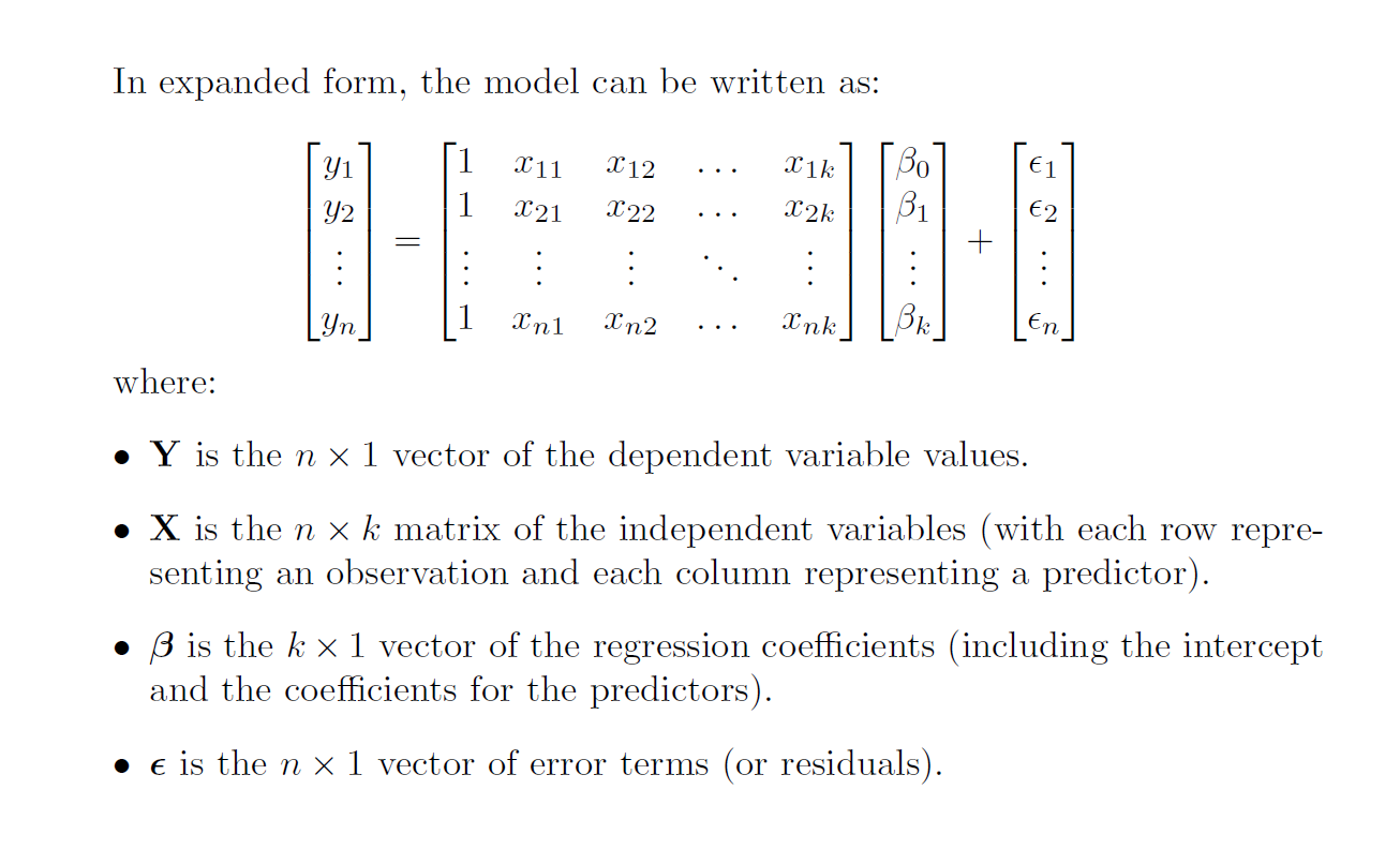

The same assumptions follow as in the simple linear regression model.

Errors must be uncorrelated with each other and errors are i.i.d conditionally normally distributed $\boldsymbol{\epsilon} \mid \mathbf{X} \sim N(0, \sigma^2 I)$.

Deriving $\boldsymbol{\hat{\beta}}$

Finding the beta now is also a different as we deal with differentiation of vector of $\hat{\beta}$. The idea is still the same, we minimize the sum of squared residuals that is now a vector.

\[\min_{\boldsymbol{\hat{\beta}}} \epsilon^T \epsilon = \min_{\boldsymbol{\hat{\beta}}} (\mathbf{Y} - \mathbf{X} \boldsymbol{\hat{\beta}})^T (\mathbf{Y} - \mathbf{X} \boldsymbol{\hat{\beta}})\]

Let us derive the $\boldsymbol{\beta}$ from the minimization problem:

\[\min_{\boldsymbol{\hat{\beta}}} (\mathbf{Y} - \mathbf{X} \boldsymbol{\hat{\beta}})^T (\mathbf{Y} - \mathbf{X} \boldsymbol{\hat{\beta}})\]

Let us shift the transpose inside, becoming as follows:

\[\min_{\boldsymbol{\hat{\beta}}} (\mathbf{Y^T} - \boldsymbol{\hat{\beta}^T} \mathbf{X^T} ) (\mathbf{Y} - \mathbf{X} \boldsymbol{\hat{\beta}})\]

One should know that changes above should hold true simply by checking matrix dimensions.

Let us expand the terms.

\[\min_{\boldsymbol{\hat{\beta}}} \mathbf{Y^T}\mathbf{Y} - \mathbf{Y^T}\mathbf{X}\boldsymbol{\hat{\beta}} - \mathbf{\boldsymbol{\hat{\beta}}^T}\mathbf{X^T}\boldsymbol{Y} + \mathbf{\boldsymbol{\hat{\beta}}^T}\mathbf{X^T}\boldsymbol{X}\mathbf{\boldsymbol{\hat{\beta}}}\]

We can now differentiate with respect to $\boldsymbol{\hat{\beta}}$.

However, we first have an intermezzo over differentiating with respect to vectors.

\[\frac{\partial \boldsymbol{\hat{\beta}}^T}{\partial \boldsymbol{\hat{\beta}}} = \mathbf{I} \quad \text{and} \quad \frac{\partial \boldsymbol{\hat{\beta}}}{\partial \boldsymbol{\hat{\beta}}} \neq \mathbf{I}\]

where

\[\boldsymbol{\hat{\beta}} = \begin{bmatrix} \hat{\beta}_1 \\ \hat{\beta}_2 \\ \vdots \\ \hat{\beta}_p \end{bmatrix}, \quad \boldsymbol{\hat{\beta}}^T = \begin{bmatrix} \hat{\beta}_1 & \hat{\beta}_2 & \dots & \hat{\beta}_p \end{bmatrix} \quad I = \text{k * k identity matrix}\]

We see that if we differentiate simply $\hat{\beta}$ with respect to $\hat{\beta}$ or column vector on column vector, the results will be invalid. The reason for this lies on the logic of differentiation.

\[\frac{d\begin{bmatrix} \hat{\beta}_1 \\ \hat{\beta}_2 \\ \vdots \\ \hat{\beta}_k \end{bmatrix}}{d\begin{bmatrix} \hat{\beta}_1 \\ \hat{\beta}_2 \\ \vdots \\ \hat{\beta}_k \end{bmatrix}} \quad \text{vs} \quad \frac{d\begin{bmatrix} \hat{\beta}_1 & \hat{\beta}_2 & \dots & \hat{\beta}_k \end{bmatrix}}{d\begin{bmatrix} \hat{\beta}_1 \\ \hat{\beta}_2 \\ \vdots \\ \hat{\beta}_p \end{bmatrix}}\]

Looking at the first way of differentiation, it would not make sense. There is no clear logic on what to differentiate for instance first term of the vector in the numerator $\hat{\beta}_1$ with respect to. It can be to $\hat{\beta}_2$ or even to $\hat{\beta}_k$.

In the second way of differentiation, we see the clear logic on what we should differentiate with respect to.

By showing differentiation by row in numerator against column in denominator, we see that the first element of the transposed $\hat{\beta}$ can be differentiated against the every $k$ elements of the $\hat{\beta}$ below which forms the first row of the identity matrix. The first element of the resulting row matrix is 1 while the rest $k-1$ elements is 0.

The second element in the transposed $\hat{\beta}$ can be differentiated in the same way to form second row of the identity matrix. The second element of the resulting row matrix will be 1 while the other $k-1$ elements will be 0.

Continuing further we will produce $k$ rows that form the identity matrix of dimensions $k * k$.

Continuining minimization of the $\boldsymbol{\hat{\beta}}$:

\[\min_{\boldsymbol{\hat{\beta}}} \mathbf{Y^T}\mathbf{Y} - \mathbf{Y^T}\mathbf{X}\boldsymbol{\hat{\beta}} - \mathbf{\boldsymbol{\hat{\beta}}^T}\mathbf{X^T}\boldsymbol{Y} + \mathbf{\boldsymbol{\hat{\beta}}^T}\mathbf{X^T}\boldsymbol{X}\mathbf{\boldsymbol{\hat{\beta}}}\]

We cancel out differentiation of the first term as there is no $\boldsymbol{\beta}$ meaning the term is $0$. Let us solve the differentiation of the remaining terms, one by one. We start with the second term up to the fourth term.

Second term:

\[\frac{d}{d\boldsymbol{\hat{\beta}}} -\mathbf{Y^T}\mathbf{X}\boldsymbol{\hat{\beta}}\]

We see that differentiation $\boldsymbol{\hat{\beta}}$ on $\boldsymbol{\hat{\beta}}$ is invalid, thus we have to transpose the objective function of differentiation to make this vector differentiation valid.

\[-(\mathbf{Y^T}\mathbf{X}\boldsymbol{\hat{\beta}})^T = -\boldsymbol{\hat{\beta}^T} \mathbf{X^T} \mathbf{Y}\]

Transposing the objective function above will not change anything. Why? $\mathbf{Y^T}\mathbf{X}\boldsymbol{\hat{\beta}}$ itself is a $1x1$ scalar if we calculate it’s dimensions. A transpose of a scalar remains the same scalar.

\[\frac{d}{d\boldsymbol{\hat{\beta}}} -\boldsymbol{\hat{\beta}^T} \mathbf{X^T} \mathbf{Y} = \frac{d\boldsymbol{\hat{\beta}^T} }{d\boldsymbol{\hat{\beta}}} -\mathbf{X^T} \mathbf{Y} = -I\mathbf{X^T} \mathbf{Y} = -\mathbf{X^T} \mathbf{Y}\]

Third term:

\[\frac{d}{d\boldsymbol{\hat{\beta}}} - \mathbf{\boldsymbol{\hat{\beta}}^T}\mathbf{X^T}\boldsymbol{Y}\]

We can directly calculate this as we are differentiating tranpose $\boldsymbol{\hat{\beta}^T}$ on $\boldsymbol{\hat{\beta}}$. There is no need to apply the transpose to the objective function.

\[\frac{d\mathbf{\boldsymbol{\hat{\beta}}^T}}{d\boldsymbol{\hat{\beta}}} -\mathbf{X^T}\boldsymbol{Y} = - I \mathbf{X^T}\boldsymbol{Y} = - \mathbf{X^T}\boldsymbol{Y}\]

Final term:

\[\frac{d}{d\boldsymbol{\hat{\beta}}} \mathbf{\boldsymbol{\hat{\beta}}^T}\mathbf{X^T}\boldsymbol{X}\mathbf{\boldsymbol{\hat{\beta}}}\]

We also see that transpose is not necessary. We can directly arrive at the differentiation that is:

\[\frac{d\mathbf{\boldsymbol{\hat{\beta}}^T}}{d\boldsymbol{\hat{\beta}}}\mathbf{X^T}\boldsymbol{X}\mathbf{\boldsymbol{\hat{\beta}}} = 2I\mathbf{X^T}\boldsymbol{X}\mathbf{\boldsymbol{\hat{\beta}}} = 2\mathbf{X^T}\boldsymbol{X}\mathbf{\boldsymbol{\hat{\beta}}}\]

The reason for the $2$ coming out is because we see that differentiation of the squared $\mathbf{\boldsymbol{\hat{\beta}}}$ will bring the power of $2$ into the front.

Combining the terms such that we satisfy the minimization procedure:

\[-\mathbf{X^T} \mathbf{Y} -\mathbf{X^T} \mathbf{Y} + 2\mathbf{X^T}\boldsymbol{X}\mathbf{\boldsymbol{\hat{\beta}}} = 0\] \[-2\mathbf{X^T}\mathbf{Y} + 2\mathbf{X^T}\boldsymbol{X}\mathbf{\boldsymbol{\hat{\beta}}} = 0\] \[2\mathbf{X^T}\boldsymbol{X}\mathbf{\boldsymbol{\hat{\beta}}} = 2\mathbf{X^T} \mathbf{Y}\]

Expressing $\boldsymbol{\hat{\beta}}$ in terms of the other factors:

\[\mathbf{\boldsymbol{\hat{\beta}}} = (\mathbf{X^T}\boldsymbol{X})^{-1} \mathbf{X^T} \mathbf{Y}\]

We can also expand this by replacing $\mathbf{Y} = \mathbf{X} \boldsymbol{\beta} + \boldsymbol{\epsilon}$

\[\mathbf{\boldsymbol{\hat{\beta}}} = (\mathbf{X^T}\boldsymbol{X})^{-1} \mathbf{X^T} \mathbf{X} \boldsymbol{\beta} + \boldsymbol{\epsilon} = (\mathbf{X^T}\boldsymbol{X})^{-1} \mathbf{X^T} \mathbf{X} \boldsymbol{\beta} + (\mathbf{X^T}\boldsymbol{X})^{-1} \mathbf{X^T}\boldsymbol{\epsilon} = \boldsymbol{\beta} + (\mathbf{X^T}\boldsymbol{X})^{-1} \mathbf{X^T}\boldsymbol{\epsilon}\]

We have derived the $\boldsymbol{\hat{\beta}}$ for multiple regression model.

Deriving distribution of $\hat{\boldsymbol{\beta}}$

We can also find the mean and variance of the $\boldsymbol{\beta}$ that can be useful to check for accuracy of beta.

\[E[\boldsymbol{\hat{\beta}} \mid X] = E[\boldsymbol{\beta} + (\mathbf{X^T}\boldsymbol{X})^{-1} \mathbf{X^T}\boldsymbol{\epsilon} \mid X] = \boldsymbol{\beta} + (\mathbf{X^T}\boldsymbol{X})^{-1} \mathbf{X^T} E[\boldsymbol{\epsilon} \mid X] = \boldsymbol{\beta} + (\mathbf{X^T}\boldsymbol{X})^{-1} \mathbf{X^T}*0 = \boldsymbol{\beta}\] \[Var[\boldsymbol{\hat{\beta}} \mid X] = Var[\boldsymbol{\beta} + (\mathbf{X^T}\boldsymbol{X})^{-1} \mathbf{X^T}\boldsymbol{\epsilon} \mid X] = (\mathbf{X^T}\boldsymbol{X})^{-1} \mathbf{X^T} Var[\boldsymbol{\epsilon} \mid X] \mathbf{X} (\mathbf{X^T}\boldsymbol{X})^{-1}\] \[\sigma^2 (\mathbf{X^T}\boldsymbol{X})^{-1} \mathbf{X^T} \mathbf{X} (\mathbf{X^T}\boldsymbol{X})^{-1} = \sigma^2 I (\mathbf{X^T}\boldsymbol{X})^{-1} = \sigma^2 (\mathbf{X^T}\boldsymbol{X})^{-1}\]

$\boldsymbol{\hat{\beta}}$ is therefore normally distributed as such:

\[\boldsymbol{\hat{\beta}} \sim N(\boldsymbol{\beta}, \sigma^2 (\mathbf{X^T}\boldsymbol{X})^{-1})\]

How does the $\hat{\beta}$ and $\boldsymbol{\hat{\beta}}$ estimates differ for both Simple and Multiple Linear Regressions?

The $\beta_1$ in the simple linear regression model simply considers the direct relationship between the predictor and the response, which can be intuitively seen in the formula $\beta_1 = \frac{cov(x_i, y_i)}{var(x_i})$

In the multiple regression model however, each $\hat{\beta_k}$ element in the row vector $\boldsymbol{\hat{\beta}}$ is calculated such that it also has been controlled for the effect of other predictors as well, and this intuitively connected to the matrix term $(\mathbf{X^T}\boldsymbol{X})^{-1}$ in the $\boldsymbol{\hat{\beta}}$ estimate. In $(\mathbf{X^T}\boldsymbol{X})^{-1}$, the multiplication between different elements of the matrix is reflective of the relationships between variables. Although not strictly a variance-covariance matrix, it is referred to as such due to the fact that it is structurally equivalent to variance-covariance matrix.

Testing accuracy of the $\boldsymbol{\beta}$

These betas are useful for the same purpose as described in the simple linear regression model, in order to conduct tests (t-tests) and obtain measures of confidence interval that can help show the accuracy of $\hat{\boldsymbol{\beta}}$.

There are slight changes to what the t-statistic and confidence interval will be constructed in the multiple regression model.

T-Tests

\[t_j = \frac{\hat{\beta}_j}{\sqrt{s^2 \cdot \left( (X'X)^{-1} \right)_{jj}}} \sim t(n-k)\]

We see some changes in the degrees of freedom. In this multiple regression model, we have k parameters (inclusive intercept), hence degree of freedoms is constrained by k parameters, meaning the independent observations become only n-k.

We also note of the structurally equivalent variance-covariance matrix $(X’X)^{-1}$. To find the t-statistic corresponding to every element in the vector $\hat{\boldsymbol{\beta}}$, we need the variance of every predictor, and this structurally lies in the diagonals of the term $(X’X)^{-1}$, hence the notation $(X’X)^{-1}_{jj}$.

Confidence Intervals

The confidence intervals remain fairly similar.

\[\boldsymbol{\beta} \quad \epsilon \quad (\hat{\boldsymbol{\beta}} \pm t_{(n-2, 1-\frac{\alpha}{2})} \cdot \text{se}(\hat{\boldsymbol{\beta}}))\]

What we see here is that we essentially calculate a vector, where each element will result in the individual confidence interval of every $\hat{\beta_j}$ of the multiple regression model.

Important Measure of General Regression Models

$R^2$: R-squared and it’s Components

We first need to understand some terms:

The total sum of squares measures the total variation of $y_i$.

\[\text{Total Sum of Squares} = \sum_{i=1}^n (y_i - \bar{y})^2\]

The regression sum of squares measures the variation explained by the regression model. It essentially finds deviation of the predicted values $\hat{y}_i$ from the mean of observed response variable $\bar{y}$.

\[\text{Regression Sum of Squares} = \sum_{i=1}^n (\hat{y}_i - \bar{y})^2\]

The residual sum of squares is something we have discussed before.

\[\text{Residual Sum of Squares} = \sum_{i=1}^n (y_i - \hat{y}_i)^2\]

The relationship between the three is as follows:

\[\text{Total Sum of Squares} = \text{Regression Sum of Squares} + \text{Residual Sum of Squares}\]

The $R^2$ of a regression model is a measure that tells us how much does the variability of the predictor variables explains variation of the response variable.

The $R^2$ is shown by this formula:

\[R^2 = \frac{\text{Regression Sum of Squares}}{\text{Total Sum of Squares}} = \frac{\text{Explained Variation}}{\text{Total Variation}}\]

A common rule of thumb is that the higher the $R^2$, the better the model explains the response variable. However, it is also wise to not consider the rule of thumb too literally, as in aiming for 90% or above. There are complex things in the world where explaning everything is simply not possible. Depending on the context, even a low $R^2$ would suffice if the aim was to find a model that can partly explain the response.

Violation of Assumptions in (Simple and Multiple) Linear Regression: Diagnosis and Solutions

It is very important to check for these violations. We need to satisfy linear regression assumptions to ensure that our beta estimate is unbiased and consistent (sure to converge to true value in large population) while being able to produce accurate inferences in tests, measuring confidence intervals and standard errors. If violations of the model occur, these inferences above can potentially be invalid as these measures heavily rely on the assumptions of the linear regression being fulfilled.

A very simple way to check if assumptions of the linear regression is violated is through checking plots of the residuals of the regression model.

Taking this example from the book of R Programming for Actuarial Science by McQuire & Kume (2020):

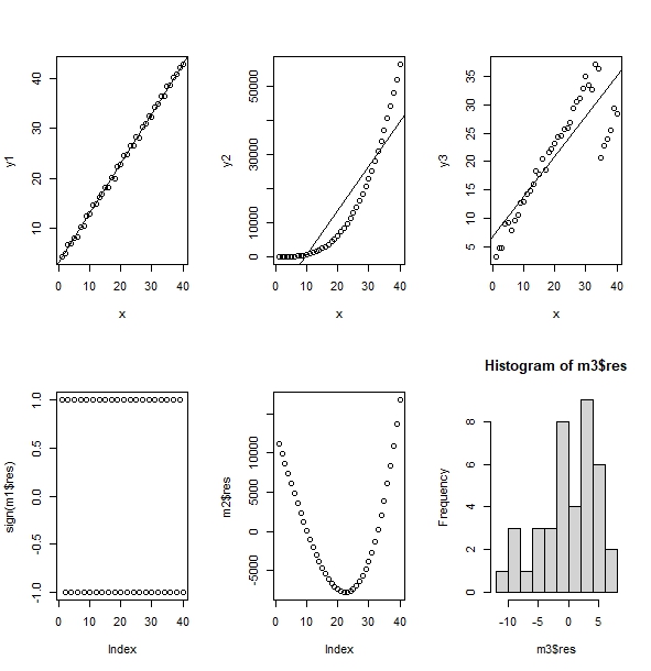
We see here examples of violations of the assumptions of the linear regression model.

Alternating signs of residuals (-1 and 1) in the first model (column 1 graphs) violates the fact that errors are independent.

In the second model (column 2 graphs) one can clearly see that linear regression does not fit the graph that is most likely quadratic.

In the third model, we clealy see that the mean of residuals is clearly not centered around zero. This violates the fact that $e_i \mid x_i \sim N(0, \sigma^2)$.

Let us go through by theory the possible depatures from assumptions of the linear regression model and the possible remedies:

Heteroskedasticity

Homoskedasticity tells us that the diagonals of the variance-covariance of errors must be constant. Heteroskedasticity is the opposite of that: when these variances of residuals are not constant. It can be that some residuals have smaller variance whilst other have larger variances and vice versa.

This can typically happen due to ommitted variable bias. If we miss out on some predictor in the model, the residuals will capture the effects of this missing variable that can exhibit some pattern leading to non-constant variance of residuals. A wrong functional form (such as in case 2 above) of trying to model a quadratic response using linear predictors can also be passed down to the residuals in the form of heteroskedasticity.

Detection

There are two ways test for heteroscedasticity:

• Graphically by plotting the residuals (x-axis) against the predicted values (y-axis) for less complex models (simple linear regression)

A common diagnosis by the graph for heteroscedasticity if we see a clear pattern, for instance increasing residuals as the predicted values increase (typically cone shaped) or if there are clear clusters in the graph. There is no heteroscedasticity if the spread of these points are randomly scattered around 0.

• Use the Breusch-Pagan test for more complex models (multiple linear regression).

The Breusch Pagan test will always follow the null hypothesis that there is no heteroscedasticity in the model.

The test first starts with a preliminary regression of the full model where it’s residuals are saved.

\[\mathbf{Y} = \mathbf{X} \boldsymbol{\beta} + \boldsymbol{\epsilon} \quad \text{then save the residuals} \quad \boldsymbol{e} = \mathbf{Y} - \mathbf{X} \boldsymbol{\hat{\beta}}\]

The auxiliary regression for this test, where we regress the squared of saved residuals from the preliminary regression on suspected predictors $Z = (z_{1i}, z_{2i}, …, z_{ki})$ that cause the heteroscedasticity, and check for whether coefficients of the predictors are zero (excluding the intercept). These suspected predictors can be from the preliminary regression, or transformations of predictors.

\[e_{i}^2 = \gamma_1 + \gamma_2 z_{1i} + \cdots + \gamma_p z_{ki} + \omega_i \quad \text{or} \quad \boldsymbol{e^{T}e} = \boldsymbol{Z} \boldsymbol{\gamma} + \boldsymbol{\Omega}\]

The idea of the auxiliary regression is to see whether the predictors explain the residuals, because if it does it is clear evidence of non-constant variance of errors.

The last step of this test calculates the of the Lagrange Multiplier test statistic of $nR^2$ that is chi squared distributed with degrees of freedom (d.o.f) $k-1$ where k is the number of predictors in the auxiliary regression and $R^2$ is the R-squared of the auxiliary regression. The idea of the auxiliary regression is to see whether the predictors explain the residuals, because if it does it is clear evidence that errors can vary, providing evidence of non-constant variance of errors. Hence if our total predictors are k (inclusive intercept), and if the intercept does not count into the test, hence the test-statistic has a d.o.f of $k-1$.

\[LM = nR^2_{\text{auxiliary}} \sim \chi^2(k-1)\]

Solution

• Robust standard errors are usually used in models with heteroscedasticity. These do not eliminate heteroscedasticity, but they produced adjusted standard errors accounted for heteroscedasticity.
• Add more variables that one could have possibly missed out on to ensure errors do not capture effect of missing variables.

Autocorrelation

The linear regression model assumes that there is no serial correlation (autocorrelation) between errors of observations, in other words the off-diagonal terms of the error terms are thus 0, making the variance-covariance of errors a completely diagonal matrix. Autocorrelation tells us that the off-diagonal terms of the variance-covariance matrix of errors of observations are not zero unlike assumed by the linear regression assumptions, telling us that there is correlation between the error terms of individual observations.

A very common occurence of autocorrelation is in time series data, where typically a response variable in this period is dependent on the response variable of the previous period. Take for instance a real life example where we want to model that can measure current price of a stock. Failing to include possible lagged values (omitted variable bias) of the historical prices may cause autocorrelation as the errors pick this up. Similar to heteroscedasticity, the incorrect functional form of the model can also cause autocorrelation.

Detection

There are two ways to check for Autocorrelation:

• Graph the autocorrelation plot (ACF plot). This plot shows the correlation between lags of the variable suspected to possess autocorrelation.

The typical ACF plot is served with a shaded blue region (or two horizontal lines that encloses a region) which can be seen as the confidence threshold that indicates evidence that correlation is significantly different from zero. If there is points that penetrate out of this blue region, it is a good indication that autocorrelation is present in one’s data. If lines are contained inside this blue region, it is a evidence that autocorrelation is contained and statistically significant at 0.

• Conduct the Breusch-Godfrey test.

A preliminary regression is first conducted on the full model where it’s residuals are saved up.

\[\mathbf{Y} = \mathbf{X} \boldsymbol{\beta} + \boldsymbol{\epsilon} \quad \text{then save the residuals} \quad \boldsymbol{e} = \mathbf{Y} - \mathbf{X} \boldsymbol{\hat{\beta}}\]

The auxiliary regression model then regresses residuals from the preliminary regression on $k$ number of lags of residuals alongside predictors of the original model. The lagged residuals can be obtained by regressing lagged $\mathbf{Y}$ i.e. $\mathbf{Y_{i-1}}$ up to $\mathbf{Y_{i-p}}$ on $\mathbf{X}$’s.

\[e_i = \mathbf{x}_i' \delta + \gamma_1 e_{i-1} + \cdots + \gamma_p e_{i-p} + \omega_i, \quad i = p + 1, \dots, n\]

This test aims to test whether coefficients of these lagged residuals are jointly equal to 0 or not. The idea is that if the lagged residuals do explain the residual then we have established that there is a relationship between errors, hence providing evidence that autocorrelation is present.

The Breusch Godfrey test follows the null hypothesis of no autocorrelation, and has the test statistic of $nR^2$ that is chi-squared distributed with degree of freedom $k$, where $k$ is the number of lags in the auxiliary regression model. Since there are $k$ number of lags to be tested in the auxiliary regression model, hence the d.o.f is k.

\[LM = nR^2_{\text{auxiliary}} \sim \chi^2(k)\]

Solution

• Add more explanatory variables, for instance lags. Recheck with relevant ACF plots if autocorrelation still exists or not.

Endogeneity

Endogeneity happens when there is correlation between the predictor and error term of the regression. This is equivalent to saying that the error term of model affects the response. This violates the assumption of fixed $x_i$’s, as they are now stochastic due to unforeseen factors that influence the $x_i$. It will be hard to therefore distinguish individual contributions of the regressor on predicted responses.

Let me elaborate a model where this can happen. Assume that we aim to simply regress wages simply on education level of the individual. However, one came to hypothesize that level of parent’s education can also affect the education level of the individual. However, it is not in the model. This therefore becomes captured in the errors. The level of education of the parent (in this case hidden in the error) will directly affect the wages.

Other possible causes of endogeneity may be due to measurement errors, omitted variable bias, or more commonly due to simultaneity of variables.

Detection

• By logical reasoning similar to the example above.

We can logically assume that level of education of an individual can be affected by level of their parents education. It is very likely that if their parents do not attend university, so likely will the child not attend university as well. Of course, one can check the validity of this relationship by a separate regression. This is why people consider the level of education as endogenous.

• If logical reasoning is unable to help us deduce (or if we need strong evidence to support the logical reasoning) we can use the Durbin-Wu-Hausman test.

The null hypothesis tells us that $k_0$ suspected endogenous regressors are exogenous, while the alternative states that $k_0$ suspected endogenous regressors are indeed endogenous.

Assume we have total of $k$ variables, where $k_0$ are endogenous and $k-k_0$ are exogenous.

The test first conducts two preliminary regressions: First of the full model (inclusive all variables, endogenous and exogenous) where all it’s residuals will be saved and the second when every suspected endogenous variable $X = (x_{k-k_0+1}, \cdots , x_{k_0})$ is regressed by the it’s potential instruments $Z=(z_1, \cdots , z_i)$ where $k_0$ vectors of residuals are saved.

\[\mathbf{Y} = \mathbf{X} \boldsymbol{\beta} + \boldsymbol{\epsilon} \quad \text{then save the residuals} \quad \boldsymbol{e} = \mathbf{Y} - \mathbf{X} \boldsymbol{\hat{\beta}}\] \[\mathbf{x_{k-k_0+1}} = \mathbf{Z} \boldsymbol{\gamma_{k-k_0+1}} + \boldsymbol{\Upsilon_{k-k_0+1}} \quad \text{then save the residuals} \quad \boldsymbol{v_{k-k_0+1}} = \mathbf{x_{k-k_0+1}} - \mathbf{Z} \boldsymbol{\hat{\gamma}}_{k-k_0+1}\] \[\cdots\] \[\mathbf{x_{k_0}} = \mathbf{Z} \boldsymbol{\gamma_{k_0}} + \boldsymbol{\Upsilon_{k_0}} \quad \text{then save the residuals} \quad \boldsymbol{v_{k_0}} = \mathbf{x_{k_0}} - \mathbf{Z} \boldsymbol{\hat{\gamma}}_{k_0}\]

In the auxiliary regression, the errors (from the full model) are regressed onto the predictors of the full model (inclusive $k_0$ endogenous variables and $k-k_0$ exogenous variables) and the $k_0$ vectors of residuals from the second preliminary model (every endogenous predictor on it’s instruments) and tests for whether coefficients of these $k_0$ vectors of residuals in the auxiliary regression is equal to 0.

If it is, then it is evidence that the suspected endogenous residuals do indeed have a relationship with the errors full model, serving as evidence for endogeneity.

\[e_i = \sum_{j=1}^{k} \delta_j x_{ji} + \sum_{j=k-k_0+1}^{k} \alpha_j v_{ji} + \zeta_i\]

This DWH-test has a test statistic of $nR^2$ that is chisquare distributed with d.o.f $k_0$. If there are $k_0$ residuals predicted from regression of every suspected endogenous variables on instruments used in the auxiliary regression whose coefficients will be tested, it therefore means there are $k_0$ coefficients to test in the auxiliary regression, hence the d.o.f of $k_0$.

\[LM = nR^2_{\text{auxiliary}} \sim \chi^2(k_0)\]

Solution

• Two Stage Least Squares Regression

The first stage attempts to first regress the suspected endogenous variable on it’s possible predictors called instruments. Instruments must satisfy the fact they are indeed relevant (logical) and are strictly correlated only with the endogenous regressor but not with the response variable (or errors) in the main model. The predicted values of the endogenous regressor are then saved. In the second stage the response variable is then regressed on the predicted values of the suspected endogenous regressor along with other predictors. The idea of this regression is to ensure isolate effects of these instruments to the main model as it is already done in the first stage. In that sense, all effects of instruments to the endogenous variable is already captured in the first stage ensuring no direct spillover effects to the main regression model.

• IV estimator

It has the same idea and purpose as the TSLS regression, the only difference that is directly incorporated as a matrix calculation of the $\boldsymbol{\beta}$.

Conclusion

In this article, I explained the underlying idea of linear regression. Specifically, I went through step by step on how to derive estimates of regression, and how to create inferential statistics out of these estimates that can useful to test for accuracy of beta. I also went through the possible violations of the regression model, it’s causes, how to detect them and solutions for it.

In the next article, I will go through applications of regression in R, stay tuned!

References

Heij, C., de Boer, P., Franses, P. H., Kloek, T., & van Dijk, H. (2004). Econometric Methods with Applications in Business and Economics. Oxford University Press.

McQuire, A., & Kume, M. (2020). R Programming for Actuarial Science. Wiley.