
Present Value
The Present Value is extremely important concept in the world of finance. In practice, this concept, by the name itself, is used very often to arrive at the current value financial products. Knowing the current value of financial products in one’s possesion is essential to quantify financial risks, and allows us to have a good overview of the health of one’s investments. In this article, I will present the concepts of the present value, and apply some coding examples in R to illustrate the applications of this concept in the real world.
Introduction to Present Value
Present value tells us the current worth of a of future receivable or to be given out cashflow (or a series of one) by discounting it to the present using the appropriate discount (interest) rates. But why the concept of present value? Why discount the value of money? It all goes back to economics. The time concept of money tells us that yearly inflation erodes the value of money. This also directly erodes the value of every financial product that obviously depends on cashflows of money. Due to this, people want to essentially estimate the value of their future money now, by using some appropriate discount rate because they know their spending power (of money) in the future will not be as powerful as now. While the discount rate may reflect predicted inflation, it also reflect other factors such as the opportunity cost of capital or risk premium, or a minimal yield that a person is willing to undertake for an investment.
This concept is easily simplified by this number line we see.
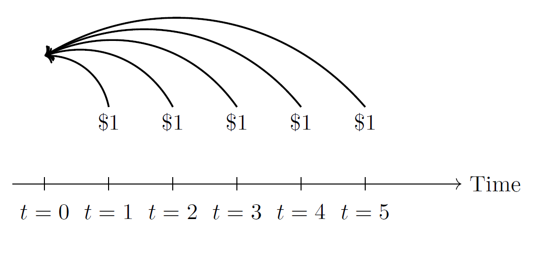
Assume that we have cashflows of 1 from $t=1$ to $t=5$. Assume that these cashflows are given at the end of the period. We are then asked to find the present value (at $t=0$) of this series of cashflows. Looking at the number line above, the goal is to discount all the cashflows (thus from $t=1$ to $t=5$) back into $t=0$. After that, we can sum up all the current values of the cashflows in the future to get the present value of the series of cashflows at $t=0$. Assume a constant discounting rate to use is 5%. The formula to do so is simplified below:
\[PV_{t=0} = \frac{$1}{(1+0.05)^1} + \frac{$1}{(1+0.05)^2} + ... + \frac{$1}{(1+0.05)^5} = $4.329477\]We can summarize the general formula of the finding the present value, of a series of n cashflows discounted back to $t=0$, assuming constant discounting rate as follows:
\[\sum_{n = 1}^{n} \frac{\text{Cashflow}_{t_n}}{(1 + i)^{t_n}}\]The $t_n$ is the arbitrary time which we want to start the discounting from. The reason I do not start with arbitrary $t$ directly in the summation, but with $t_n$ instead, is due to the fact that the time variable in this formula may vary based on the way that cashflows may be received/given out. This will be further elaborated on the later sections. The $t_n$ belonging to the discounting factor can generally be seen as a sequence of differences between the time of the cashflow minus the time to which we want to discount back to.
If we are asked to find the PV at t=0 using the constant force of interest, it is quite straightforward as well:
\[\sum_{n = 1}^{n} {\text{Cashflow}_{t_n}}e^{-\int_{t_1 = 0}^{t_2 = n} \delta \ ds}\]We should note variations to the formula. If the discounting rate is variable, the notation should be changed to $\delta_{t_n}$.
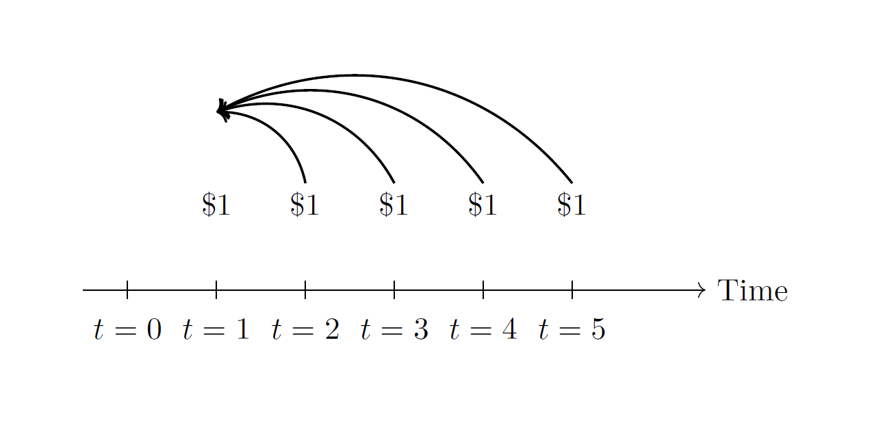
Now, what if I want to calculate the present value of the same cashflow series (paid at the end of the period) above in the picture, assuming same constant discounting rate of 5%, but at $t=1$? What this means is that cashflows in between $t \in (0,1]$ will be ignored. Why? The cashflow of 1 has been received/given out at $t=1$, thus it is not further in our interest to find the present value of 1 of $t=1$ as it has been received. What we now focus on is the cashflows in $t \in (1,5]$, or the cashflows from $t=2$ to $t=5$. The purpose of present value is to calculate the current value of all cashflows to be given to or received in the future. Calculating the present value thus becomes as illustrated by the number line:
\[PV_{t=1} = \frac{$1}{(1+0.05)^1} + ... + \frac{$1}{(1+0.05)^4} = $3.545951\]However, note that the above can only apply for the present values of $t=0$ to $t=4$. If we assume with the picture above that the cashflow ends at $t=5$, and we want to find the value of the present value at $t=5$. What then? This should make sense because we do have to calculate the present value at every possible time point to get an complete overview of things. There is esentially no future cashflows after $t=5$, but we still have to find a value for it. The present value at $t=5$ is therefore no other than our cashflow at $t=5$, that is 1. There is no discounting as we attempt to find the present value at $t=5$, of the cashflow at $t=5$ at the same time.
This is a quick overview of the concept of the present value along with motivation of its use. In the next section, I will explain how this concept of present value is simplified in Actuarial Science.
The annuity: an actuarial concept that uses the present value
In Actuarial Science, there is a concept of annuity that embeds the concept of present value. The annuity is a notation that tells us the sum of present values of a set of future cashflows of unit 1 for a given time period. There are various notations to this annuity that reflects the different ways the 1 unit cashflows are being received or given out which I briefly touched upon. This is again the reason why $t$ starts and ends at different time values for the different annuities below. Below I show examples of types of annuities.
Immediate annuity or annuity in advance:
\[\ddot{a}_{\overline{n}|}^{@i} = \sum_{t = 1}^{n} \frac{\text{Cashflow}}{(1 + i)^t}\]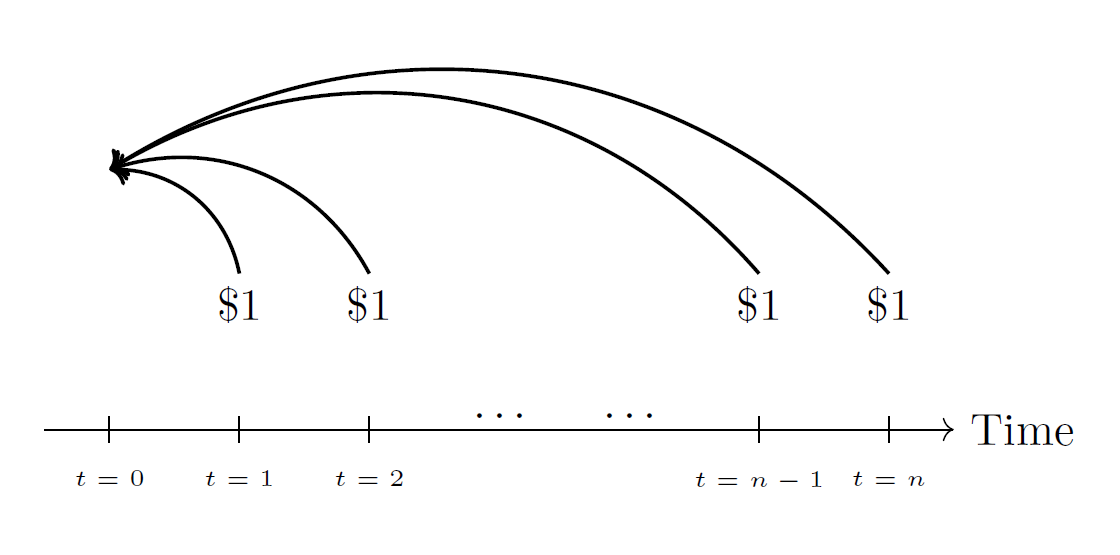
This notation tells us that the cashflows in question are given out at the end of the period, starting from $t=1$ up until arbitrary time $t=n$. It gives the present value to $t=0$ of the series of 1 unit of cashflows, discounted by constant $i$, as shown in the picture above.
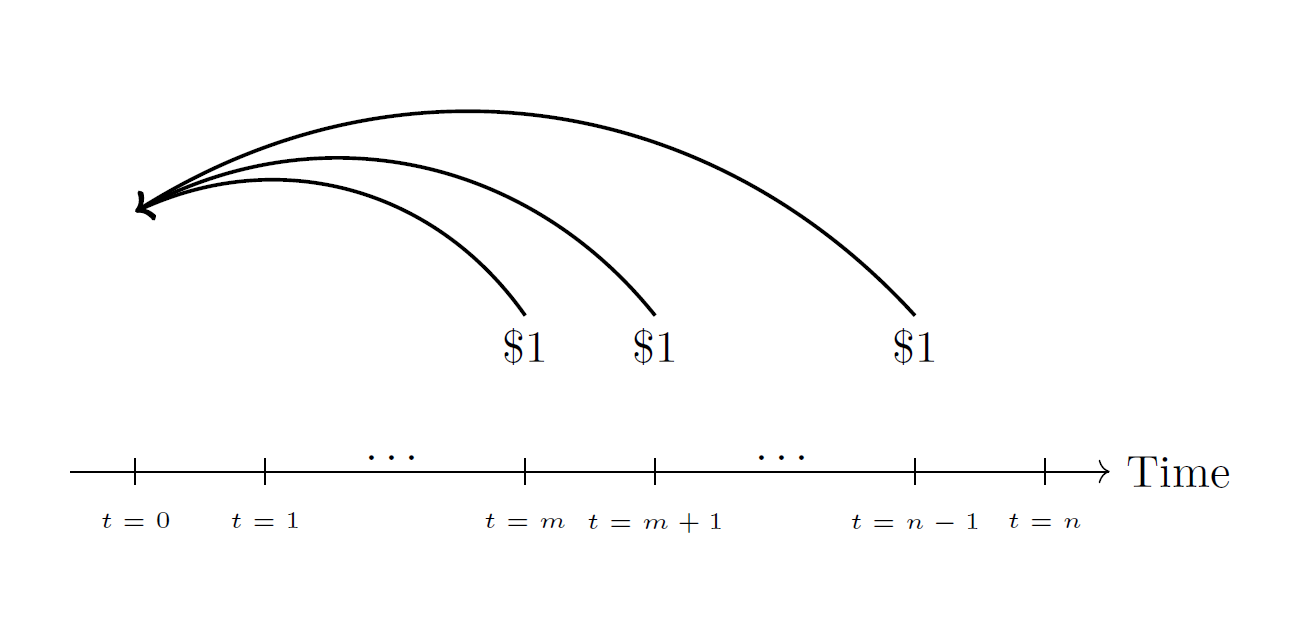
Annuity due or annuity in arrears:
\[a_{\overline{n}|}^{@i} = \sum_{t = 0}^{n-1} \frac{\text{Cashflow}}{(1 + i)^t}\]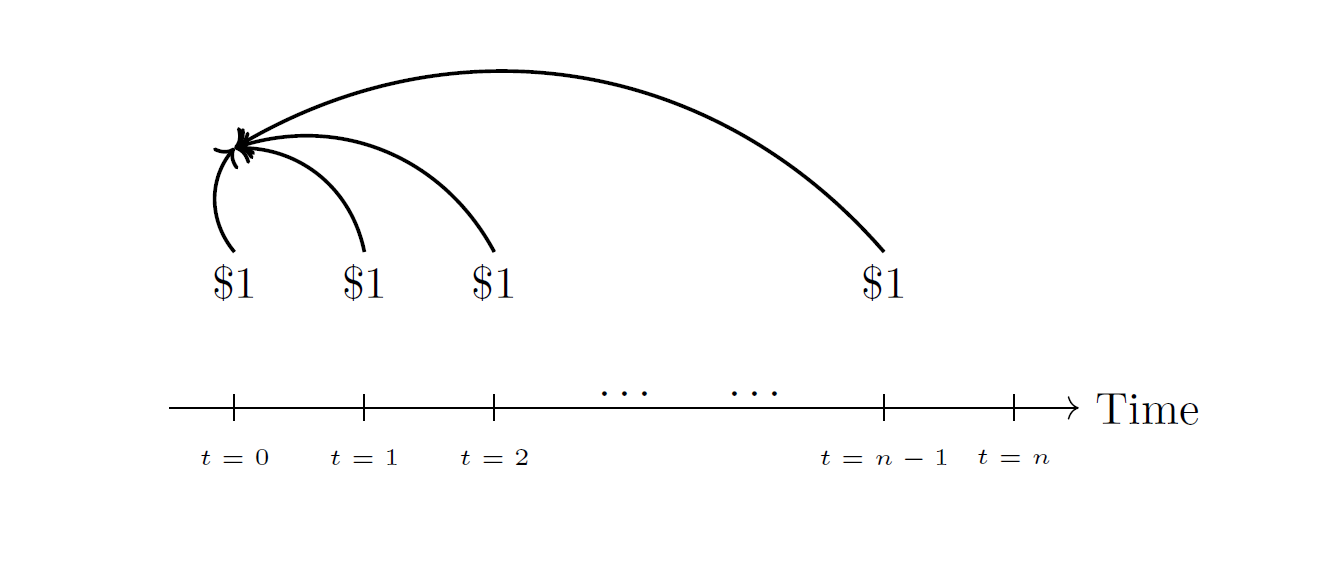
This notation tells us that the cashflows in question are given out directly at the beginning of the period, starting from $t=0$ up until arbitrary time $t=n-1$. It calculates the sum of all the present value of same amount of cashflows above in the picture discounted by constant $i$. Note here we also calculate the present value of the cashflow at $t=0$, which shall logically remain as 1.
Deferred annuity in arrears and in advance
I am not able to reproduce the notation of the deferred annuity in arrears using MathJax. However, the difference is not much. We simply add $m \vert$, where $m$ is the deferment period, to the left subscript of the notation for annuity in arrears, to get deferred annuity in arrears equation. A deferment period of $m$ a m-period of delay before the payment of 1 unit starts at or after $t=m$, which in the case of cashflow in arrears, should start at $t=m+1$, after $t=m$.
\[\text{Deferred Annuity in Arrears} = \sum_{t = m+1}^{n} \frac{\text{1}}{(1 + i)^t}\]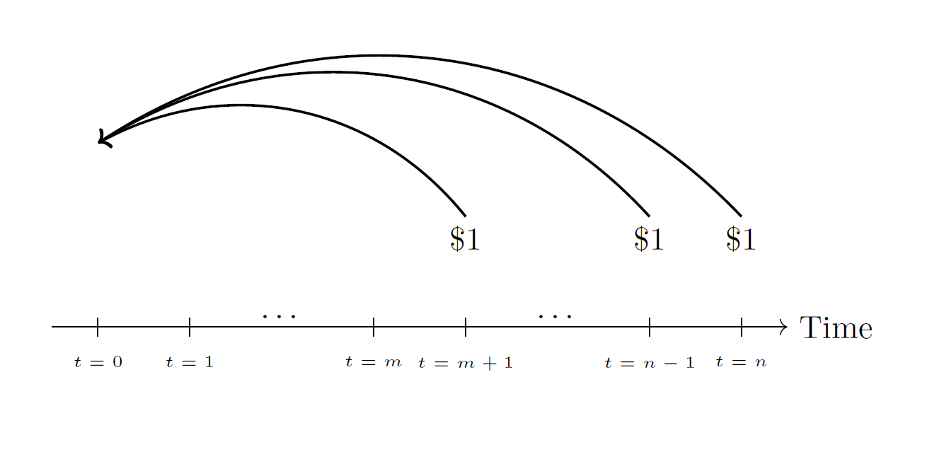
We see that cashflows start at $t=m+1$ up until $t=n$ and these are discounted back to $t=0$, the present.
For deferred annuity in advance, cashflows are given out or received at the beginning of the period. The only difference in cashflow to the image above, is that the first cashflow starts directly at the beginning of $t=m$ and ends at $t=n-1$, shown in the picture below.
Special Case: p-thly annuities
What if we are faced with cashflows of $p$ frequencies per annum? What does the notation become? What happens to our calculations? Let us take an example of an monthly annuity in arrears.
\[a_{\overline{n}|}^{(p)@i} = \sum_{t = 1}^{n*p} \frac{\frac{\text{1}}{p}}{(1 + \frac{i^{(p)}}{p})^t}\]The differences are clear and understandable. The nominal interest rate of one unit interval that has been adjusted for frequency $p$, $\frac{i^{(p)}}{p}$ should be used to reflect the nominal rate per discrete $p$-thly intervals. The cashflow itself has also been scaled down by $p$ in order to reflect the true cashflows of the of p-thly interval. The time intervals are also chopped into in $p$-thly intervals further. What we do in the end is the same, it is just a matter of summing up the present values of each $\frac{1}{p}$ cashflows of smaller intervals.
Other Types of Annuities
There are more types of annuities in practice. Think of continuous annuities, increasing or decreasing annuities. These will not be further discussed here, and can be easily read online. The concept of these to the ones above remain the same, these are notations to tell us the sum of present values of a specific set of cashflows.
Present Value Function and Constructing Annuity Function in R
In this section I will show you how to build up a function in R that calculates value of an annuity, using the built in presentValue() function. To understand this section it is assumed the reader has familiarity with R to some degree.
Built-in function of presentValue
In the “lifecontingencies” package, the presentValue() function is extremely handy to simplify present value calculations. However, we should note a downside to this built-in function. We can only use the effective rate here. Thus, if we are given force of interest, it should be changed into the effective rate before it can be plugged into presentValue(). Using “?presentValue” documentation, we are able to see the different input parameters. Simply plugging in the cashflow vector, time vector, and interest rate (vector, if applicable) into the function already allows us to find the present value easily as shown below. Below is an example.
install.packages("lifecontingencies")
library(lifecontingencies)

# Construct a random increasing step cashflow
cashflow <- seq(1,10)
# Construct a random time sequence for the discounting factor
time <- seq(0,9)
# Input a random effective rate for discounting; assumes constant rate of i for all time intervals
i <- 0.05
# Plug everything into presentValue()
presentValue(cashflow, time, i)

[1] 41.34247
Annuity Code
Now, I will now construct a single function to calculate both annuity in arrears and in advance, accounting for payment frequency. Look and try to understand the descriptions of each line of code.
# Note the inputs: the effective rate (i), the term of the annuity (n), the frequency of payments # (p), and type that is a logical input (0: arrears or 1: advance) to tell the function if we are # calculating annuity in advance or annuity in arrears.


annuity_function <- function(i, n, p, advance){
  #Construct cashflow of annuity, accounting for p-thly intervals.
  cashflow <- rep(1/p, each=n*p)
  #Construct time intervals for the discounting factor for annuity in arrear back to t=0, considering p.
  time_arrear <- seq(1, n*p, 1)
  #Construct time intervals for the discounting factor for annuity in advance back to t=0, considering p.
  time_advance <- seq(0, n*p-1, 1)
  #Change the effective rate into nominal rate suitable for p-thly intervals
  i_p <- (1+i)^(1/p) - 1
  #Calculate the value of the annuity given the inputs (either arrear or advance)
  annuity_value <- ifelse(advance == 1, presentValue(cashflow, time_advance, i_p), presentValue(cashflow, time_arrear, i_p))
}

# Value of a 1 unit 10-year annuity in arrears, with monthly payment frequency
annuity_function(0.04,10,12,0)
# Value of a 100 unit 10-year annuity in arrears, with monthly payment frequency (simply mutiply function above by 100)
100*annuity_function(0.04,10,12,0)
# Check validity of the function by comparing it to built in function annuity()
annuity(i = 0.04, n = 10, m= 0, k = 12, type="arrears")

[1] 8.258543
[1] 825.8543
[1] 8.258543
I tried to find the present value of a 10-year annuity in arrears discounted at a effective rate of 4%, with a monthly payment frequency. The steps are clear: construct the cashflow, time intervals, and effective rate, input all into the presentValue() function, before plugging all those into function I built.
Now, let us try to add a deferred input into the function now (for advance and arrears), which builds up from the previous code:
# The inputs remain the same as the previous code, except for the addition
# of the variable m, that is the deferment period.

deferred_annuity <- function(i, n, m, p, advance){
  #Construct cashflow of annuity, accounting for p-thly intervals.
  cashflow <- rep(1/p, each = n*p)
  #Construct the annuity in arrear time vector for the discounting factor back to t=0 when the cashflow start paying out after deferment
  time_arrear <- seq(m*p + 1, (m+n)*p, 1)
  #Construct the annuity in advance time vector for the discounting factor back to t=0 when the cashflow start paying out after deferment
  time_advance <- seq(m*p, (m+n)*p - 1, 1)
  #Change the effective rate into nominal rate suitable for p-thly intervals
  i_p <- (1+i)^(1/p) - 1
  #Calculate the value of the annuity given the inputs (either arrear or advance)
  pres_val <- ifelse(advance == 1, presentValue(cashflow, time_advance, i_p), presentValue(cashflow, time_arrear, i_p))
}

# Find the present value at t=0 of an 3-year deferred annuity of length 10 years, subject to monthly payments, and has interest rate of 4%
deferred_annuity_function(0.04,10, 3, 12, 0)
[1] 7.341814

# Validate if function is correct using built-in annuity function
annuity(i = 0.04, n = 10, m= 3, k= 12, type="arrears")
[1] 7.341814
We can see that it is not that complex either. We simply need to incorporate $m$ into the previous function, which changes the content of the time intervals, as shown in the deferred annuity function. It could be possible that you will not directly arrive at the function above, hence it is always wise to construct the annuity function step by step. For instance, first without considering frequency payments, then with frequency payments, then with the deferrment period.
We have seen that building the annuity function is not hard to construct. Again, simply define your cashflows, the time sequence, and interest rates, plug them into presentValue() function, and voila!
Note that it would be wise to cross-check your function with the results of the built-in function of annuity() of the “lifecontingencies” package for the validity of the function coded. Additionally, it is also advised to experiment building different annuity functions out there, for instance of increasing or decreasing annuities.
Valuing Financial Products for Asset Liability Management as an Application of Present Value: Loan and Bond Value Calculation Example in R
One important application of the presentValue() is in Asset Liability Management. As I have briefly touched upon in the excerpt, this presentValue() can allow us to calculate the health of one’s investments in financial products, and potentially allow for decision making to purchase or sell financial assets. In this section I will give examples on how we can visualise the value of a financial product over time, using the presentValue() and annuity function, which is the essence of asset liability management.
Loan Value Derivation
The annuity function coded in the previous section can be useful to value some financial instruments that may have a constant cashflow. An example is a loan schedule.
Assume that we have received a traditional loan schedule of this characteristics:
- The loan has a value of $1$ million
- It is to be repaid back in $10$ years alongside an effective interest of $5$% per annum.
- The payment structure can be arranged, such that every year we pay the same amount that covers both the interest and the capital at the end of the period (in arrears).
To find the payment structure every year, we can use actuarial equivalence which asks us to find the equal n yearly repayments whose sum of it’s present value will equate to the original loan amount of $1000000$.
\[\text{Repayment}*a_{\overline{n}|}^{@i} = \text{Loan Amount} \rightarrow \text{Repayment} = \frac{\text{Loan Amount}}{a_{\overline{n}|}^{@i}}\]# Define loan characteristics
loan_amount <- 1000000; interest <- 0.05; term <- 10; p <- 1
# Use actuarial equivalence on the annuity function we created earlier:
repayment <- loan_amount/annuity_function(0.05, 10, 1, 0)
To find the value of the loan at every yearly interval during it’s life, we simply deduct the annuity term every year by 1 multiplied by the repayment amount. This esentially gives us the amount of loan (value of loan) still due to the receiver by the borrower at every year until the loan maturity.
# Construct vector of loan values every year
loan_value <- NULL

# Construct for loop to find the annuity
for(i in seq(term,1,-1)){
  loan_value[term+1-i] <- repayment*annuity_function(0.05, i, 1, 0)
}
loan_value

# The value of the loan at t=10 is naturally 0 because we assumed the loan has been fully paid off at t=10 with the loan schedule.
# The for loop does not catch this, so we have to manually add 0 to the end of the loan value vector
loan_value <- c(loan_value, 0); loan_value

# Construct table of loan
table_loan <- data.frame("Time" = 0:term, "Loan_Value_at_t" = loan_value); table_loan

    Time Loan_Value_at_t
1     0       1000000.0
2     1        920495.4
3     2        837015.6
4     3        749361.8
5     4        657325.3
6     5        560687.0
7     6        459216.8
8     7        352673.1
9     8        240802.2
10    9        123337.7
11   10             0.0
To see whether this repayment structure makes sense or not, we can manually construct separate elements of the loan schedule above to check this.
# Check the elements of the loan schedule from t=0 to t=10
# We want to see whether this repayment schedule does indeed already cover all the outstanding loans and
# the interests associated to it
# There is the element of loan_outstanding, loan_paid, and interest_paid
loan_outstanding <- NULL; interest_paid <- NULL; loan_paid <- NULL
for (i in 1:term){
  # The loan at t=0 is the original loan amount
  loan_outstanding[1] <- loan_amount
  # The interest paid is the interest rate multiplied by the current outstanding loan, which
  # decreases by year as we pay off the loan capital
  interest_paid[i] <- interest*loan_outstanding[i]
  # We assumed part of the repayment consists of the payment of interest and payment of loan,
  # thus, to find the loan amount paid, we subtract the repayment with the interest paid at t
  loan_paid[i] <- repayment - interest_paid[i]
  # The outstanding loan left at the next period is naturally the outstanding loan amount in the previous
  # period subtracted by the loan paid in the previous period
  loan_outstanding[i+1] <- loan_outstanding[i]-loan_paid[i]
  # The for loop only produces loan_paid and interest_paid up to i=9, because outstanding_loan at t=10 is already 0 as shown.
  # This already confirms that our repayment structure does indeed work in repaying the whole loan plus interest
  # To complete things, we have to manually add 0 as the last elements in both of the vectors mentioned.
  loan_paid[term+1] <- 0
  interest_paid[term+1] <- 0
}

# Table of the loan schedule from t=0 to t=10
# We add the repayment vector along the table, to allow us to see that this repayment does
# indeed equal to the loan paid plus interest paid for each time period from t=0 to t=10
data.frame("Time" = 0:10, "Outstanding Loan"= round(loan_outstanding,2), "Loan Paid"= loan_paid,
           "Interest Paid" = interest_paid, "Repayment" = c(rep(repayment, each=term), 0))

    Time Outstanding.Loan Loan.Paid Interest.Paid Repayment
1     0        1000000.0  79504.57     50000.000  129504.6
2     1         920495.4  83479.80     46024.771  129504.6
3     2         837015.6  87653.79     41850.781  129504.6
4     3         749361.8  92036.48     37468.091  129504.6
5     4         657325.3  96638.31     32866.267  129504.6
6     5         560687.0 101470.22     28034.352  129504.6
7     6         459216.8 106543.73     22960.841  129504.6
8     7         352673.1 111870.92     17633.654  129504.6
9     8         240802.2 117464.47     12040.108  129504.6
10    9         123337.7 123337.69      6166.885  129504.6
11   10              0.0      0.00         0.000       0.0
Through this loan schedule, we can see that the repayment structure works perfectly fine, and therefore the annuity function can indeed be used as a much more simpler method to calculate the value of a loan. A interesting point to note here is that the loan and interest payment structure in each repayment differs. As we pay off the loan capital slowly, it is logical that the interest amount we are going to pay decreases in proportion of the repayment, which in turn increases the loan amount proportion in the repayment as time passes until the maturity.
Knowing how to calculate the loan value at certain points in time is important for asset management. Assume that a bank has a loan portfolio and wishes to know the value of their loans (or how much loans do their borrowers still owe them) at some point in time. I will use the loan portfolio dataset arrived from the book R Programming for Actuarial Science by McQuire and Kume to illustrate on how to calculate one’s loan portfolio (the total value of loans outstanding).
# First, load the dataset. Make sure to fit the code below to fit your directory
Loans100<- read.csv("~/Loans100_for_exercise.csv")
# Shows the contents of the csv file
head(Loans100)
  Loan.number Intial.loan Term Agreed.rate Start.date..1.Jan.
1           1      320000    2       0.026               2020
2           2      520000   13       0.049               2017
3           3      650000   23       0.048               2020
4           4      570000   12       0.048               2010
5           5      480000   12       0.022               2018
6           6      430000   18       0.042               2019

tail(Loans100)
95           95      140000   19       0.033               2016
96           96      790000   14       0.047               2017
97           97      930000   20       0.047               2016
98           98      230000   22       0.045               2017
99           99      380000   24       0.039               2017
100         100      700000   18       0.040               2020

# Construct a function that uses the columns of the Loan100 function (that is Loan100[i]),
# that contains characteristics of the loan, but we use q[] to represent an arbitrary csv dataset.
# It follows the same code as earlier, which is now adjusted a little.
year_of_interest <- 2021
outstanding <- function(q){
  # Construct first the null vectors of the loan schedule elements
  outstanding_loan <- NULL
  interest_paid <- NULL
  loan_repaid <- NULL
  # q[3] or Loan100[3], if one checks, is the column of the time to maturity of bond
  time <- seq(0, as.numeric(q[3]))
  for(i in 1:as.numeric(q[3])){
    # q[2] or Loan100[2] is the loan amount
    outstanding_loan[1] <- as.numeric(q[2])
    # Calculates yearly repayments of the individual loan schedules in the portfolio
    p <- as.numeric(q[2])/annuity(as.numeric(q[4]), n=as.numeric(q[3]), type="arrears")
    # q[4] or Loan100[4] is the column of interest rates agreed in each loan schedule
    interest_paid[i] <- outstanding_loan[i]*as.numeric(q[4])
    loan_repaid[i] <- p - interest_paid[i]
    outstanding_loan[i+1] <- outstanding_loan[i]-loan_repaid[i]
    loan_repaid[as.numeric(q[3])+1] <- 0
    interest_paid[as.numeric(q[3])+1] <- 0
  }
  # Constructs a table that shows the loan value development of ONE loan
  df <- data.frame(time, round(outstanding_loan,2), interest_paid, loan_repaid, c(rep(p, as.numeric(q[3])),0))
  # This is a if function that tells us if the loan in question has already matured in 2021, it will return 0,
  # as the loan value that is matured, is obviously 0. While loans that have not matured in 2021, will be
  # considered and their element will plucked out of the dataframe that shows loan value development
  # and that shows the loan value in 2021
  ifelse(year_of_interest > as.numeric(q[3])+as.numeric(q[5]), 0, df[year_of_interest-as.numeric(q[5])+1, 2])
}
# The built-in apply function applies every row of the Loan100 csv dataset into the function, and returns every
# loan value of each loan at 2021 if applicable (remember the if function above that filters out the loans
# that have matured in 2021)
x <- apply(Loan100, 1, outstanding); x
  [1] 162053.31 392849.89 633915.40  60674.72 371483.43 396385.42 615368.73 170758.12 277870.34 377538.96 101097.75
 [12] 495151.71 436304.79 661951.25 460987.44 496298.07 527597.08 474340.07 405392.65 421199.59 528752.60 785780.90
 [23] 881155.75 451112.97 196854.32 544671.17 794181.27 513412.23 337819.94 694016.49 118523.35 244217.67 335018.73
 [34] 513747.88 378288.95 705479.10 507207.77 697078.13 409885.29 646438.90 682784.45 624971.16 634469.03 112274.56
 [45] 330052.26 544159.61 378245.95 486590.22 200433.44 583416.42 492423.86 689129.83 532002.81 404208.39 764176.24
 [56] 490786.26 509013.31 152451.13  90133.33 333288.98 695905.32 141850.76 544211.08 122544.96 966559.58 125186.33
 [67] 693639.28 609369.14 610045.70 125235.04 641950.67 801525.31 200467.03 740654.53 537106.10 255740.63 664072.61
 [78] 904470.05 743848.54 446704.46 271442.19 328564.14 616048.12 232656.20 800250.44 273858.53 449750.20 812704.46
 [89] 604547.33 452113.07 571897.80 646000.62 164736.42 171392.39 111076.25 613404.31 770553.92 202895.53 338241.03
[100] 672704.67

sum(x)
[1] 46933798

# Of course, if one is interested in finding the sum of their loans every year onwards, they can use a for loop
# to change the year of interest in the line ifelse(year_of_interest > as.numeric(q[3])+as.numeric(q[5]), 0,
# df[year_of_interest-as.numeric(q[5])+1, 2]) of 2021 into 2022, 2023, and further.

# I am interested in calculating value of loans of the portfolio from 2021 to 2040

xx <- NULL
for(i in 2021:2040){
  year_of_interest <- i
  # To tidy up the matrix dimensions, make sure it starts from 1st element up to last element,
  # not from the 2021th element to 2045th element.
  xx[i-2020] <- sum(apply(Loans100, 1, outstanding))
}

# Gives sum of loan values of the portfolio from 2020 up to 2040
xx
 [1] 46933798 43894236 40967909 37927472 34768098 31484742 28072130 24524748 21196191 18003762 15001798 12447732
[13] 10182781  8155268  6406811  4765972  3459815  2408741  1731569  1116183
We can see that this code succesfully calculates the loan value of a portfolio of loans, and gives us a good overview of amount of loans left that one can receive. Of course, this assumes that all loans are paid accordingly when the time comes to pay. In real life, this might not happen, and thus codes above can be adjusted to calculate loan values in the circumstances mentioned above.
Bond Value Derivation
In another instance, the annuity function might not help us, because our annuity function above does not take into account non-constant cash flows unlike the loan schedule above. Take a bond for example. It is assumed that the reader knows the basics of a bond.
Assume we want to find a values over time of a coupon bearing bond with these characteristics:
- A face value of $400$
- Coupon rate payment of $10$%, giving coupon payments of $40$ every year including at the maturity.
- Assume increasing interest rates starting from $3$% at $t=1$, and increasing $0.5$% yearly. This means that if our cashflows are at $t=1$, $t=2$ we must discount it by $3$% and $3.5$% respectively, and so on. We can assume this reflects the expected return that has been set for this particular bond.
As how a normal bond payment is structured, for the $n-1$ years we will only receive cashflow of coupon payments. In the last cashflow at maturity $n$, we will be paid out the coupon payment along with the face value $F+c$. We also logically assume that these cashflows are paid at the end of the period. To find the present value at $t=0$, we can code as below:
# Define characteristics of bond: 20-year-bond of face value 100, with coupon rate of 6%, and interest vector assumed above:
face_value <- 400; coupon_rate <- 0.1; coupon <- face_value*coupon_rate; term <- 20; interest <- seq(0.03, by=0.005)

# Calculating the bond value at t=0:

# Define cashflows of bond as described:
bond_cashflow <- c(rep(coupon, each=term-1), face_value + coupon)
# Define the time of cashflows of the bond, assumed payments are made in arrears
bond_time <- seq(1,term)

# Use presentValue to find bond value at t=0
presentValue(bond_cashflow, bond_time, interest[1:length(bond_cashflow)])

[1] 430.4872
And so, we arrive at the value of the bond at $t=0$. This is the present value of all future cashflows yet to happen after $t=0$. Now, what about the value of the 20-year-bond at $t=1$? In this case, the first coupon payment has elapsed, hence this is not in our interest to calculate it’s present value further. Now, we simply focus on the remaining cashflows: $18$ further coupon payments, and $1$ payment of the coupon plus face value, starting at $t=2$ and ending at $t=20$. To find the time vector for the discounting factor, find the difference of the time of the cashflows relative to the starting time of $t=1$. This creates a new time sequence factor starting from $t=1$ to $t=19$. With the same logic, we can imagine how the cashflows and the time vector are structured for the bond value at $t=2$, $t=3$, up to $t=20$. I will show you the code that produces a vector of the bond value starting from $t=0$ up to it’s maturity at $t=20$. We should note that at $t=20$, our present value equates to $F+c$ as we receive $F+c$ at exactly $t=20$, thus discounting this cashflow back to $20$ means the discounting factor is $1$.
# Create a bond cashflow function which produces the cashflow to find the value of bond at arbitrary t
bond_cashflow <- function(time){
  cf <- c(rep(coupon, each=time-1), face_value + coupon)
}

# Create a time vector function for the discounting factor to find the value of the bond at arbitrary t
bond_time <- function(time){
  time <- seq(1,time)
}

# Create an empty vector to store the bond values
value <- NULL

# Used a for loop to calculate the values of the bond from t=0 to t=19
for(i in 1:term){
  value[i] <- presentValue(bond_cashflow(term+1-i), bond_time(term+1-i), interest[i:term])
}

# Note of the i and term+1-i; these are parts of the code are vital to ensure the correct values are returned
# It follows my explanation of how the cashflow and time vectors are structured for values at t=0 up to t=19.
# The bond value at t=20 will be manually added to create a new complete bond value vector from t=0 to t=20.

# Returns the values of the bond from t=0 to t=20
bond_value <- c(value, face_value + coupon)

[1] 430.4872 419.0653 408.7146 399.4070 391.1215 383.8436 377.5648 372.2825 367.9995 364.7234 362.4664 361.2442
[13] 361.0759 361.9825 363.9864 367.1094 371.3715 376.7883 383.3686 391.1111 440.0000


# Construct data frame to show table of values of the bond at every t
df <- data.frame("t" = 0:20, "Bond_Value_at_t" = bond_value); df

         t   Bond_Value_at_t
1        0   430.4872
2        1   419.0653
3        2   408.7146
4        3   399.4070
5        4   391.1215
6        5   383.8436
7        6   377.5648
8        7   372.2825
9        8   367.9995
10       9   364.7234
11      10   362.4664
12      11   361.2442
13      12   361.0759
14      13   361.9825
15      14   363.9864
16      15   367.1094
17      16   371.3715
18      17   376.7883
19      18   383.3686
20      19   391.1111
21      20   440.0000

# Plot the bond value from t=0 to t=20
plot(1:length(bond_value), bond_value, type="p", pch=8, xlab="Time", ylab="Value", main="Value Growth of Bond")
We arrive at the bond value plot of below:
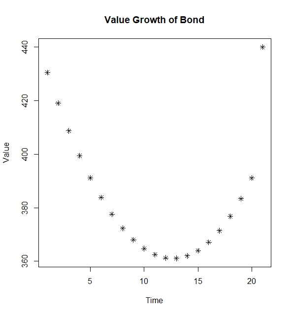
The curvature of the plot tells us the dynamic nature of the bond value when subjected to non-constant interest rates, which we assumed here.
One might wonder how can the data above be useful for in the concept of Asset Liability Management. Consider the scenario explained below:
- Assume that at $t=0$, a company is offered to buy 10,000 bonds in question above at a par with the present value at $t=0$.
- They want to consider this offer if they see that purchasing $10,000$ of this bond, amounting to $4,304,872$ can help them pay off their company debt of around $10$ million dollars that shall be due on $t=16$, assuming the increasing discount rates that they have projected. It is assumed that they keep the coupons received from the bonds, and will use it to pay the loan back. This coupons are therefore not subjected to discounting.
- In other words, they will consider the offer IF their bond investment at $t=16$ (that is their money earned from sale of the bond plus their coupons earned up to $t=16$) equals to $14,304,872$.
To be able to answer this question, we first have to modify the bond value vector derived, by adding the coupon payments already received at each time t.
# Construct a vector that shows how many coupon payments have been received from t=0 up to t=20.
coupons_received <- NULL
# Construct for loop that gives the coupon payments received so far at t=1 up to t=19
for (i in 1:term-1){
  coupons_received[i] <- coupon*i
}
# The coupon payments at t=0 and t=20 are not well defined with the for loop above. We have to edit the bond value vector to fit the context above.
# At t=0, the coupon payments we have received is still zero, hence we add 0 into the vector for the coupon payment vector
# At t=20, we have calculated the bond value as the face value plus the coupon payment together. Instead of adding 800,
# that is 40 coupon payment * 20 terms to this last element, we add 760, showing instead we have received 19 coupon payments at t=20.
coupons_received <- c(0, coupons_received, coupons_received[term-1]); coupons_received

# Returns bond_value at time t=0 to t=20 inclusive of the coupons received so far at t
bond_value_with_coupons <- bond_value + coupons_received; bond_value_with_coupons

# Constructs table to show the bond values inclusive coupons received
df2 <- data.frame("t" = 0:20, "Bond_Value_with_Coupons_at_t" = bond_value)

    t   Bond_Value_with_Coupons_at_t
1   0                     430.4872
2   1                     459.0653
3   2                     488.7146
4   3                     519.4070
5   4                     551.1215
6   5                     583.8436
7   6                     617.5648
8   7                     652.2825
9   8                     687.9995
10  9                     724.7234
11 10                     762.4664
12 11                     801.2442
13 12                     841.0759
14 13                     881.9825
15 14                     923.9864
16 15                     967.1094
17 16                    1011.3715
18 17                    1056.7883
19 18                    1103.3686
20 19                    1151.1111
21 20                    1200.0000
If we look at the value of the bond at $t=16$ with the coupons the company has received so far up to $t=16$ with the $10,000$ bonds, we see that the amount that the company now holds from the coupons plus the fee they will get if they sell the bond now with the price equalling to it’s present value at $t=16$, will be around $1011.3715*10000 = 10,113,715$. This clearly is far off from the $14,304,872$ which the company must expect to receive from their bond investment to pay off their debt of $10$ million at $t=16$. Thus, the conclusion for the company is that it will not be wise to take up the offer.
Conclusion
I have attempted to explain the concept of present value, as well as the annuity notation that incorporates the present value, which is widely used in Actuarial Science. To get a peek at the importance of this concept, I showed how we can use the present value and annuity functions created in R for real-world applications, especially in asset liability management. I hope this article has been an informative one!
References
McQuire, A., & Kume, M. (2020). R Programming for Actuarial Science. Wiley.
R-Script Download
The R-Script, along with the dataset, can be downloaded from the assets directory in my GitHub repository. The R code is under the folder “codes”, named Presentvalue_Rcode_Actuary492.R and the dataset lies under the folder “dataset”, named Loans100_for_exercise.csv
Leave a comment