Interest Rates

Interest rates. Something that we have encountered multiple times during our finance classes and in our daily lives. Examples of interest rates are coupon rates in bonds, or forward rates in derivatives. Essentially, the interest rate tells us the percent growth of an amount of fund $X_t$ at some time t over a specified time period, typically in the next year. This concept is very useful especially for actuaries in order to calculate cashflows of their client’s portfolios in order to get a good overview of their financial risk. In this article, I will bring to you the different interest rates around financial literature that can be useful to actuaries.

Effective Interest Rates and It’s Downsides

Effective interest rate (per unit time, i.e. 10% per annum) tells us that the end of a time period, the fund $X_t$ will grow by 10% to $X_{t+1}$. Essentially, we can consider this as a simple interest rate where we assume that the interest is paid at the end of the year. This can be visualized by the formula below.

\[X_1 = X_0(1+i)\]

However, this concept is quite flawed in it’s essence. Sure, it is easy and more intuitive for the average person by saying that the interest will be paid out at the end of year in our example for instance. However, in this concept of effective interest rates, we are not able to calculate the growth of a fund $X_t$ at any time between that one time period (i.e. calculating the fund at $t=0.06$ between $0<t<1$) except for the amount at the end of the time period. Thus, this interest rate concept is regarded as discrete in nature. Essentially, the fund amount in any $t$ between $0<t<1$ will therefore still remain at the original amount of $X_t$ because at $t=0.06$, we have not received the interest yet, but we will rather receive the interest at $t=1$ based on this concept. This assumption can or cannot be true - we do not know. Let’s take an example where this might not be true. We open a savings account that gives us interest of 3.5% per annum. Sure, we know directly that at the end of the year the fund in our savings will rise by 3.5%. However, logically speaking, we also know that at every second, minute, hour within that one year, interest is building up. Yet, we are not able to calculate them simply by using effective interest rates.

This concept thus can be handy if actuaries are only interested in cashflows only at certain time periods. But in some cases, actuaries can be expected to calculate fund growth in much more specific periods, such as within seconds, minutes, or hours. But, this concept of effective interest rates will not be able to fulfill such task. Now comes the question, which type of interest rate can do this?

Force of Interest and It’s Applications

It is no other than the force of interest. The force of interest, that is usually denoted as $ \delta_{t}$ can be considered as the interest earned in an “infinitesimally” small time interval. This force of interest can be variable (in terms of $t$) or be constant (i.e. 0.05). A variable force of interest, that can allow us to calculate force of interest at some future time point is also called as the forward interest rate.

I will illustrate two methods, with a step-by-step proof to show how can we use the force of interest to calculate the growth of some fund $X_t$.

This is the first method. It starts with this reasoning. The interest $\delta_{t}$ earned in a small time interval $dt$ from a fund of $X_t$, is equivalent to the increase in fund $X_t$ denoted as $dX_t$, which can be visualised as follows:

\[X_t * \delta_{t}\ * dt = dX_t\]

Rearranging the equation, with $\delta_{t}$ as the subject, we get as follows:

\[\delta_{t} \ = \frac{1}{X_t} * \frac{dX_t}{dt} = \frac{X'_t}{X_t}\]

At this point, we should be aware that the fund $X_t$ can be a function that calculates the amount of fund at some time $t$, which can be also denoted as $X(t)$. This renders the equation above as:

\[\delta_{t} \ = \frac{X'_t}{X_t} = \frac{X'(t)}{X(t)}\]

Now, I want to show the second method to get into the equation above before we move on further. Let us start with this number line:

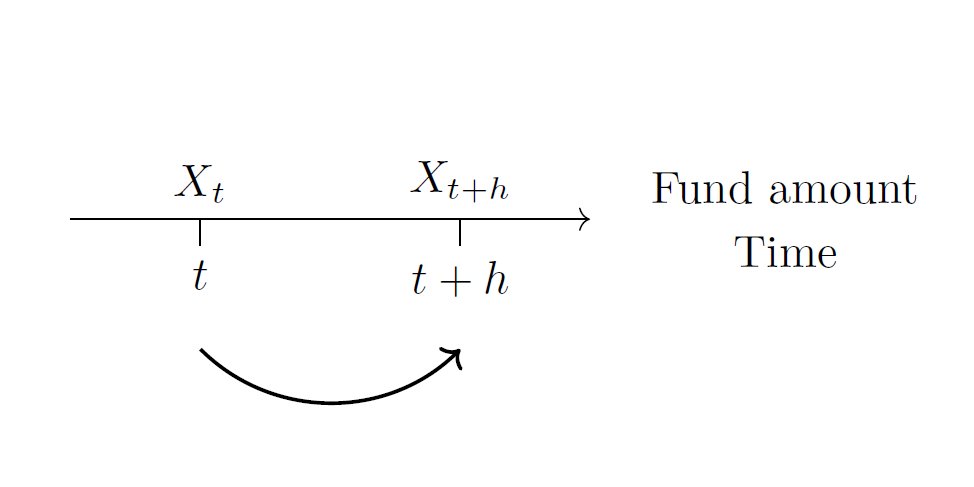
This number line tells us the growth of fund $X_t$ [ $X(t)$ ] over a time interval $h$ to $X_{t+h}$ [ $X(t+h)$ ]. The interest earned in this time interval, following simple interest rate definition, can be visualised as:

\[i[t, t+h] = \frac{X(t+h) - X(t)}{X(t)}\]

Now, let us assume that we can chop up more intervals in between $t$ and $t+h$ until $h$ becomes infinitesimally small. This also directly translates to chopping up the interest rate accrued between $t$ and $t+h$, that is $i[t, t+h]$, into $h$ infinitesimally small intervals, towards the limit where $h \rightarrow 0$, to give us the interest rate at infinitesimally small intervals, which we also know is the definition of the force of interest $\delta$.

This equation described above is illustrated below as:

\[\delta_t = \lim_{h \to 0} \frac{i[t, t+h]}{h} = \lim_{h \to 0} \frac{\frac{X(t+h) - X(t)}{X(t)}}{h} = \lim_{h \to 0} \frac{X(t+h) - X(t)}{h} * \frac{1}{X(t)}\]

Remembering the limit definition of a derivative below:

\[\lim_{h \to 0} \frac{f(x+h)-f(x)}{h} = f'(x)\]

We can then simplify the proof as follows by using definition of derivative:

\[\lim_{h \to 0} \frac{X(t+h) - X(t)}{h} * \frac{1}{X(t)} = \frac{1}{X(t)} * \lim_{h \to 0} \frac{X(t+h) - X(t)}{h} = \frac{X'(t)}{X(t)} = \delta_{t}\]

We have now seen that this also arrives at the same equation that equates force of interest earlier above in the first method.

\[\delta_{t} = \frac{X'(t)}{X(t)}\]

It is important to understand the reasoning behind how both methods are able construct the equation relating to the force of interest. Now, in order to see how the fund evolves with the force of interest, we have to express $X(t_2)$, that is the fund at some arbitrary new time $t_2$, in terms of $X(t_1)$, the original fund amount at some arbitrary time $t_1$ and in terms of $\delta_{t}$.

We now start with the equation we just derived below:

\[\delta_{t} = \frac{X'(t)}{X(t)}\]

Next, let us integrate both sides in some time interval $t_1$ to $t_2$:

\[\int_{t_1}^{t_2} \delta_{t} \ ds = \int_{t_1}^{t_2} \frac{X'(s)}{X(s)} \, ds\] \[\int_{t_1}^{t_2} \delta_{t} \ ds = \left[ ln(X(s)) \right]_{t_1}^{t_2}\] \[\int_{t_1}^{t_2} \delta_{t} \ ds = ln(X_{t_2}) - ln(X_{t_1}) = ln(\frac{X_{t_2}}{X_{t_1}})\]

Now, we can simply rearrange the equation above to express $X_{t_2}$ in terms of $X_{t_1}$ and $\delta_{t}$.

\[\int_{t_1}^{t_2} \delta_{t} \ ds = ln(\frac{X_{t_2}}{X_{t_1}})\] \[e^{\int_{t_1}^{t_2} \delta_{t} \ ds} = \frac{X_{t_2}}{X_{t_1}}\] \[X_{t_2} = X_{t_1} * e^{\int_{t_1}^{t_2} \delta_{t} \ ds}\]

Looking at the equation above, we can clearly see that the interest rate is not exactly the force of interest, but rather the equation that is:

\[e^{\int_{t_1}^{t_2} \delta_{t} \ ds}\]

To find the discounting rate using the force of interest, simply add a negative behind the integral of the function above:

\[e^{-\int_{t_1}^{t_2} \delta_{t} \ ds}\]

This interest accumulation equation itself, based on the force of interest, is very important in the world of financial mathematics. With this equation, even if we are given a force of interest that is per annum, we are still able to calculate the interest that shall be accrued between time intervals of minutes, days, or hours and this solves the limitation of the effective interest rates. This is further embedded into logic by the integral in the equation, which tells us that we are esentially calculating the sum of infinitesimally small time intervals of interest rates between some arbitrary time period. The integral also explains the continuous nature of this force of interest, and why people regard the force of interest also as the continuous interest rate.

Let us take an example where we need to calculate the interest of borrowing $100 000$ in 10 days time for one day, given an constant annual force of interest of $\delta = 0.05$ . By the accumulation formula based on the force of interest, it should be fairly simple. We first have to adjust the annual $t$ into daily time interval by dividing by $365$. What this means is that we are interested in the fund growth between time $t_1=10/365$ and $t_2=11/365$. Plugging this into the accumulation function of the force of interest:

\[X_{t_2} = X_{t_1} * e^{\int_{t_1}^{t_2} \delta_{t} \ ds}\] \[X(11/365) = X(10/365) e^{\int_{10/365}^{11/365} 0.05 \ ds} = 100000 e^{\int_{10/365}^{11/365} 0.05 \ ds} \approx 100013.7\]

We therefore see that the interest of borrowing $100 000$ for 1 day in the 10th day is about $13.70$ based on this concept. Looking back, this is something we could not have calculated with only the effective interest rates

Let us visualise another equation where we assume instead of fixed cash flows, we have continuous cashflows, and we want to find the present value (PV) of these cashflows. Let us say we want to calculate the present value at $t=0$ of a cashflow in between arbitrary times $t_1$ and $t_2$. The formula to do so thus simply becomes:

\[PV = \int_{t_1}^{t_2} \rho(t)e^{-\int_{0}^{t} \delta_{s} \ ds} \ dt\]

When we use fixed or continuous cashflows, the formula essentially still stays the same, except that now, cashflows that are now dependent on $t$. Therefore, the cashflow equation must logically speaking, be sent inside the integral, before solving for the integral to get the PV.

I want to explain the inner and outer integral bounds, which may be confusing. First, the reason for inner integral bound of the force of interest to be from $0$ to $t$ is because we are interested in finding the PV at $t=0$, thus we have to adjust the force of interest to find the accumulating discounting factor from $t=0$ until some arbitrary time $t$ when the cashflow payments starts. This arbitrary $t$ is then made clear in the outer integral bounds, which in our case, we are interested in finding PVs of cashflows starting between $t_1$ and $t_2$. In essence, what we are then doing with this inner integration is simply first defining the accumulating discounting factor, by adjusting the integral bounds to the time of interest which we want to discount the cashflows back to, before we use it to calculate the PV of all infinitesimally small cashflows over some time period through the outer integration.

So, to visualise variations to this equation, if we are expected to find the PV of continuous cashflows at some point in time between $t=19$ and $t=20$ discounted back to $t=1$, this means the bounds of the inner integral changes to between $1$ and $t$, while the outer integral bound changes to between $19$ and $20$. Assuming the cashflows and force of interest are still unknown, the PV equation becomes:

\[PV = \int_{19}^{20} \rho(s)e^{-\int_{1}^{t} \delta_{s} \ ds} \ dt\]

The Relationship between Force of Interest and Effective Interest Rates

Taking a glance back, it was argued earlier how effective interest rates are not able to calculate interest built up in between a time period, while the force of interest is able to do so. The latter is definitely desired, however in the real world, actuaries are only often served effective interest rates, which they can only make use of to calculate growth of funds over smaller time intervals. Thus, finding the relationship between effective rates and the force of interest essentially serves as a bridge between theory and practice. In order to do this, we have to assume equality between the two different interest accumulation functions: consider two types of interest accumulated at the same time interval $0<t<1$, one using the constant force of interest (to simplify calculations) is equivalent to the other interest accrued using the effective interest rate.

Let us first equate the accumulation functions of the force of interest and effective rate:

\[X(1) = X(0)e^{\int_{0}^{1} \delta \ ds} = X(0)*e^{\delta}\] \[X(1) = X(0)*(1+i)\]

Equating the two accumulation functions:

\[e^{\delta} = (1+i)\]

This gives us an extremely important relationship. Starting with a fund of $1$, applying $\delta$ to infinitesimally small time intervals, then calculating the interest accrued over these time intervals, gives us $(1+i)$ in the end. What this also implies is that the $i$ that we derive from $\delta$ using this equation receives the continuous compounding effect due to the equality assumed, meaning $i$ can directly be applied to extremely small (non-integer) time intervals, despite the $\delta$ being calculated as per annum for instance. This may allow for more straightforward calculations.

Nominal Interest Rates

Previously, we interpreted effective interest rates as the interest received at the end of one period. The nominal interest rates ($i^{(p)}$) essentially has the same idea as effective interest rates, except that this concept can be interpreted as receiving interest more than once per unit period, where $p$ can be seen as the frequency of payments in that one unit period. For example, if $p=2$ it tells us that 2 payments are made in one unit period (i.e. 2 half-yearly payments in one year). Nominal rates are still discrete in nature, however they allow us to calculate interest rates of smaller discrete time intervals. The relationship between effective and nominal rates is as follows:

\[i^{(p)} = p((1+i)^{\frac{1}{p}} - 1)\]

Giving a quick rearrangement we can see:

\[\frac{i^{(p)}}{p} = ((1+i)^{\frac{1}{p}} - 1)\]

The nominal rate essentially tells us that some effective interest rate per unit period can be convertible or compounded into a much smaller unit period. In the rearranged equation, simply plugging in the effective interest rate, we are already able to obtain the nominal rate that is already adjusted for the payment frequency $p$, that is $\frac{i^{(p)}}{p}$.

With the above in mind, we have to be careful and note that $i^{(p)}$ is still not the rate that has been converted to fit the payment frequency, but rather the adjusted one-period interest that has been compounded p-times, and thus has to still be divided by payment frequency $p$ to get the nominal rate adjusted for payment frequency. Thus, we have to differentiate between $i^{(p)}$ and $\frac{i^{(p)}}{p}$, and recognise which one should ultimately be used based on our needs.

To put this concept into example, let’s say we need to calculate present value of monthly payments. However, we are only given that the adjusted annual nominal rate that is 0.1 per annum ($i^{(12)} = 0.1$) which has been compounded monthly. By dividing $i^{(12)}$ by 12, that becomes $\frac{0.1}{12} \approx 0.0083 $, we get the nominal rate for the monthly time interval which we then can ultimately use to calculate the present value of monthly payments. However, to be clear once again, due to the discrete nature of nominal rates, we are still not able to calculate the growth of fund at some arbitrary time point in between the monthly time periods.

When are Effective Interest Rates and Force of Interest Used?

Effective rates are used often in the world of finance due to the frequent occurences of regular and discrete of cashflows such as premiums or benefits that are only given out normally at the end of a time period, typically at the end of month. As these cashflows occur at fixed time intervals, using an effective rate consistent whose period is consistent with the frequency of payments suffices to reflect financial risk in practice. In this case, there is no need to call upon the force of interest. However, in situations where patterns of interest rates or payments are irregular and/or continuous in nature, the force of interest will be needed for calculations.

Using mortality rates as an example which you might have encountered some time in your academics, if we are only required to measure death rates between discrete time intervals, then mortality rate suffices. However, if we are asked to measure death rates over non-integer time ranges, such as the probability of survival an 80.2 year old in the next 2.5 years, the force of mortality will be better suited for this purpose.

Conclusion

In this article, we have learned about the different types of interest rates used by actuaries, it’s characteristics, and in which situations are these types of interest rates used. I hope you have learned something from this article. See you on the next one!

References

McQuire, A., & Kume, M. (2020). R Programming for Actuarial Science. Wiley.