Diversification

Diversification is very common in finance. The main purpose of diversification is to ensure that risks are significantly reduced. Financial institutions, such as banks, hedge funds and pension funds have their own diversification policies to prevent large value losses in their assets. In this article, we will explore what is diversification in mathematical terms and give an example of an application in R.

What is diversification?

Diversification may come in different forms but it’s main purpose remains the same, that is to reduce risks. What risks though?

Take for example, diversification in hedge funds and pension funds. They typically have assets in different asset classes such as stocks, bonds, and real estate whose returns have been proven by research to have very little correlation with one another. This reduces the risk of asset value loss. How? If the stock market was bearish, there may be an inflow of funds into bonds that may increase price of bonds, offsetting the temporary loss of stock value during it’s bearish phase.

For insurance companies, they diversify their policyholder portfolio by making it as large as possible. A large portfolio of carefully chosen policyholders (they go through an underwriting process pick the least risky policyholders) ensure that financial losses of the portfolio (by means of total claims) become as predictable as possible, in the process reducing the risk of extreme claims.

Of course, the diversification process which I described in these two scenarios also have to be backed up by data and expertise, which institutions such as hedge or pension funds, and insurance companies possess. Having these prerequisites allows them to create extremely reliable predictions which they can use to support their diversification policy and actions.

Diversification can also apply to the average person. In investing, we are always advised to never put our eggs in one basket, that is why people diversify their investment in different asset classes!

The mathematical intutition behind diversification

Let us express the concept of diversification mathematically.

Let us first express the return of a portfolio of n assets:

\[R_p = w_1 R_1 + w_2 R_2 + \dots + w_n R_n = \sum_{i=1}^{n} w_i R_i\]

where $w_i$ is the weight of each asset in the portfolio and these individual weights have to sum up to 1 ($\sum_{i=1}^{n} w_i = 1$). $R_i$ is seen as the return on each individual asset $i$ while $R_p$ is seen as the return of portfolio that can be seen as the sum of return of weighted assets.

Two metrics which we can attain from this portfolio return is the mean of returns and also the variance of returns. The mean can be simply seen as the average returns of the portfolios based on the weighting of each asset. The variance on the other hand should be interpreted as the risk of return of the given portfolio.

These two measures come hand-in-hand. Ideally, one wants to ensure a high mean return with the least variance (or risk) as possible but in real life this is hard to achieve. More on this will be highlighted in the next article about Modern Portfolio Theory.

We can easily find the mean of the portfolio return as follows:

\[E[R_p] = E[w_1 R_1 + w_2 R_2 + \dots + w_n R_n] = E[\sum_{i=1}^{n} w_i R_i] = \sum_{i=1}^{n} E[w_i R_i] = w_1 E[R_1] + w_2 E[R_2] + \dots + w_n E[R_n]\]

The variance of the portfolio return on the other hand looks more complex:

\[\text{Var}(R_p) = \text{Var}(w_1 R_1 + w_2 R_2 + \dots + w_n R_n) = \sum_{i=1}^{n} \sum_{j=1}^{n} w_i w_j \text{Cov}(R_i, R_j) = \sum_{i=1}^{n} w_i^2 \text{Var}(R_i) + \sum_{i=1}^{n} \sum_{\substack{j \neq i}}^{n} w_i w_j \text{Cov}(R_i, R_j)\]

where we see two important terms, that is $\text{Cov}(R_i, R_j)$ that is the covariance between asset $i$ and asset $j$ and $\text{Var}(R_i)$ is the variance of asset $i$ itself.

Although the equation looks complex, the underlying idea behind the result of the variance is very simple.

First, why can we say that the variance is the risk of return? Remembering the equation of variance:

\[\text{Var}(R) = \sum_{i=1}^{n} (R_i - E[R])^2\]

The variance itself is the dispersion of returns around their expected value. This dispersion can be seen as uncertainty or the risk associated with the return. Of course, this uncertainty in our case of portfolio, is not only the risk in each individual assets that is the variance, but also the risk between STRICTLY DIFFERENT asset pairs in the portfolio that is called the covariance.

Having the variance and covariance terms of the every individual weighted assets in the portfolio, let us express them by a variance-covariance matrix. This matrix makes the representation of risk much easier to grasp because it essentially presents all the possible ‘dispersions’ between ALL possible STRICTLY DIFFERENT return pairs (we call this covariance), including itself (we call this variance).

\[\text{C} = \text{Var-Cov Matrix} = \begin{bmatrix} \text{Var}(R_1) & \text{Cov}(R_1, R_2) & \dots & \text{Cov}(R_1, R_n) \\ \text{Cov}(R_2, R_1) & \text{Var}(R_2) & \dots & \text{Cov}(R_2, R_n) \\ \vdots & \vdots & \ddots & \vdots \\ \text{Cov}(R_n, R_1) & \text{Cov}(R_n, R_2) & \dots & \text{Var}(R_n) \end{bmatrix}\]

The first row starts with all the possible variance and covariance terms beginning with $R_1$, that is the covariance of $R_1$ with itself, which is equivalent to it’s variance, then continuing with covariance of $R_1$ with $R_2$ up to $R_n$. The second then starts in a similar fashion with variance and covariance terms beginning with $R_2$, here we first start with the covariance of $R_2$ with $R_1$, afterwards the covariance of $R_2$ with itself $R_2$ that is the variance of $R_2$, then covariance of $R_2$ with $R_3$ up to $R_n$. And so on for the third row up to the n-th row.

Doing this repeatedly forms the complete n$x$n variance-covariance matrix which we see all variance terms are located in the diagonals, and covariance terms in the off-diagonals.

Now, let us add the weight vectors to make it align with the portfolio variance equation, because we are dealing with $w_1 R_1$ up to $w_n R_n$ weighted assets returns in the portfolio return instead of simply unweighted asset returns of $R_1$ up to $R_n$.

One might wonder why is there a transpose? The idea is that the weightings of assets $w$ which are constants, are squared when taken out of the variance terms (i.e. $\text{Var}(w_1 R_1) = {w_1}^2 Var(R_1)$). This similarly applies to the covariance terms (i.e. $\text{Cov}(w_1 R_1, w_2 R_2) = w_1 w_2 Cov(R_1, R_2)$). The use of weight vectors reflect this perfectly.

\[\text{Var}(R_p) = \text{Var}(w_1 R_1 + w_2 R_2 + \dots + w_n R_n) = w^{T}Cw\]

Perhaps a more easier way to follow is indeed by directly applying the weighted random returns of individual assets directly into the variance-covariance matrix as follows, which will produce the same result as the equation above:

\[\text{C}_w = \begin{bmatrix} \text{Var}(w_1 R_1) & \text{Cov}(w_1 R_1, w_2 R_2) & \dots & \text{Cov}(w_1 R_1, w_n R_n) \\ \text{Cov}(w_2 R_2, w_1 R_1) & \text{Var}(w_2 R_2) & \dots & \text{Cov}(w_2 R_2, w_n R_n) \\ \vdots & \vdots & \ddots & \vdots \\ \text{Cov}(w_n R_n, w_1 R_1) & \text{Cov}(w_n R_n, w_2 R_2) & \dots & \text{Var}(w_n R_n) \end{bmatrix}\]

which is equivalent to

\[= \begin{bmatrix} w_1 w_1 \text{Var}(R_1) & w_1 w_2 \text{Cov}(R_1, R_2) & \dots & w_1 w_n \text{Cov}(R_1, R_n) \\ w_2 w_1 \text{Cov}(R_2, R_1) & w_2 w_2 \text{Var}(R_2) & \dots & w_2 w_n \text{Cov}(R_2, R_n) \\ \vdots & \vdots & \ddots & \vdots \\ w_n w_1 \text{Cov}(R_n, R_1) & w_n w_2 \text{Cov}(R_n, R_2) & \dots & w_n w_n \text{Var}(R_n) \end{bmatrix}\]

If we look closely at the portfolio return variance expression earlier, we can see that it is simply the sum of all the variance and covariance terms of the variance-covariance matrix that has been weight-adjusted by inclusion of weight vectors $w^{T}Cw$. We have a separate summation term for all variance terms $\sum_{i=1}^{n} w_i^2 \text{Var}(R_i)$, then another separate summation for the covariance terms $\sum_{i}^{n} \sum_{\substack{j=1 \ j \neq i}}^{n} w_i w_j \text{Cov}(R_i, R_j)$, whose extra summation of $\sum_{\substack{j=1 \ j \neq i}}^{n}$ ensures that there is no covariance term of the same asset return (i.e. $cov(R_i, R_i)$) because those are essentially the variance terms that have already been reflected in the first summation.

Special case of Variance of Portfolio Return : Equal Asset Weighting $\frac{1}{n}$

A good way to put our understanding of the concept of risk of portfolio return into the test is by checking the case when we deal with equal asset weightings $w_1 = \dots = w_n = \frac{1}{n}$. The idea on using equal asset weighting ensures that calculations are made as simple as possible, which we will show later.

But first let us find the mean and variance (risk) of portfolio returns where assets are equally weighted:

\[\text{E}(\frac{R_1}{n} + \frac{R_2}{n} + \dots + \frac{R_n}{n}) = \frac{1}{n}(\text{E}(R_1) + \dots + \text{E}(R_n))\]

We can see finding the mean of returns is quite straightforward.

\[\text{Var}(\frac{R_1}{n} + \frac{R_2}{n} + \dots + \frac{R_n}{n}) = \frac{\overline{\text{Var}(R_i)}}{n} + \frac{(n - 1) \overline{\text{Cov}(R_i, R_j)}}{n}\]

The result variance of equal-weighted assets portfolio return on the other hand is not that obvious at first glance. Let us break the steps down on how we can arrive there.

However, the idea behind calculating the variance is still the same as explained previously, it is equivalent to the sum of all terms of the equal-weighted portfolio return variance-covariance matrix. First, let us create the variance-covariance matrix when assets are equally weighted:

\[\text{C}_w = \begin{bmatrix} \text{Var}\left(\frac{R_1}{n}\right) & \text{Cov}\left(\frac{R_1}{n}, \frac{R_2}{n}\right) & \dots & \text{Cov}\left(\frac{R_1}{n}, \frac{R_n}{n}\right) \\ \text{Cov}\left(\frac{R_2}{n}, \frac{R_1}{n}\right) & \text{Var}\left(\frac{R_2}{n}\right) & \dots & \text{Cov}\left(\frac{R_2}{n}, \frac{R_n}{n}\right) \\ \vdots & \vdots & \ddots & \vdots \\ \text{Cov}\left(\frac{R_n}{n}, \frac{R_1}{n}\right) & \text{Cov}\left(\frac{R_n}{n}, \frac{R_2}{n}\right) & \dots & \text{Var}\left(\frac{R_n}{n}\right) \end{bmatrix}\]

which is equivalent to

\[= \begin{bmatrix} \frac{1}{n^2} \text{Var}(R_1) & \frac{1}{n^2} \text{Cov}(R_1, R_2) & \dots & \frac{1}{n^2} \text{Cov}(R_1, R_n) \\ \frac{1}{n^2} \text{Cov}(R_2, R_1) & \frac{1}{n^2} \text{Var}(R_2) & \dots & \frac{1}{n^2} \text{Cov}(R_2, R_n) \\ \vdots & \vdots & \ddots & \vdots \\ \frac{1}{n^2} \text{Cov}(R_n, R_1) & \frac{1}{n^2} \text{Cov}(R_n, R_2) & \dots & \frac{1}{n^2} \text{Var}(R_n) \end{bmatrix}\]

Now, let us group the summation into the variance and covariance terms.

Let us first start with the variance.

Looking at the matrix above, we see that the variance terms are only located in the diagonals. Because we have $n$ rows, this means that we have $n$ diagonal terms. Summing these diagonal terms is therefore as follows:

\[\frac{1}{n^2} \text{Var}(R_1) + \frac{1}{n^2} \text{Var}(R_2) + \dots + \frac{1}{n^2} \text{Var}(R_n) = \frac{1}{n^2} \sum_{i=1}^{n} \text{Var}(R_i)\]

How do we get the average of variance from this? As we can see:

\[\frac{1}{n^2} \sum_{i=1}^{n} \text{Var}(R_i) = \frac{1}{n} \frac{1}{n} \sum_{i=1}^{n} \text{Var}(R_i) = \frac{1}{n} * (\frac{1}{n} \sum_{i=1}^{n} \text{Var}(R_i)) = \frac{1}{n} \overline{\text{Var}(R_i)} = \frac{\overline{\text{Var}(R_i)}}{n}\]

Now, let us move on to the summation of the covariance terms.

We should remember, that there are now $n^2 - n = n(n-1)$ covariance terms. There are a total of $n^2$ terms based on the n by n variance-covariance matrix. We then substract by ‘n’ terms because we do not want to count the variance terms in the diagonals that are already in the first summation earlier. Let us now create a summation for these terms:

\[\sum_{i}^{n} \sum_{\substack{j=1 \\ j \neq i}}^{n} \text{Cov}(\frac{R_i}{n}, \frac{R_j}{n}) = \sum_{i}^{n} \sum_{\substack{j=1 \\ j \neq i}}^{n} \frac{1}{n^2} \text{Cov}(R_i, R_j) = \frac{1}{n^2} \sum_{i}^{n} \sum_{\substack{j=1 \\ j \neq i}}^{n} \text{Cov}(R_i, R_j)\]

Now, let us see how can we manipulate the equation derived above to get the average of covariances:

\[\frac{1}{n^2} \sum_{i}^{n} \sum_{\substack{j=1 \\ j \neq i}}^{n} \text{Cov}(R_i, R_j) = \frac{1}{n} \frac{1}{n} \sum_{i}^{n} \sum_{\substack{j=1 \\ j \neq i}}^{n} \text{Cov}(R_i, R_j)\]

We see that to create the average, we need to add the term $\frac{1}{n(n-1)}$ to the covariance summation because we have concluded earlier that there are $n(n-1)$ covariance terms! We also have to compensate for this term by adding $\frac{n(n-1)}{1}$. Doing these steps as shown below will lead us to the final answer:

\[\frac{1}{n} \cdot \frac{1}{n} \sum_{i=1}^{n} \sum_{\substack{j=1 \\ j \neq i}}^{n} \text{Cov}(R_i, R_j) = \frac{1}{n} \cdot \frac{1}{n} \cdot \frac{n(n-1)}{1} \cdot \frac{1}{n(n-1)} \sum_{i=1}^{n} \sum_{\substack{j=1 \\ j \neq i}}^{n} \text{Cov}(R_i, R_j) = \frac{1}{n} \cdot \frac{1}{n} \cdot \frac{n(n-1)}{1} \cdot \left(\frac{1}{n(n-1)} \sum_{i=1}^{n} \sum_{\substack{j=1 \\ j \neq i}}^{n} \text{Cov}(R_i, R_j) \right) = \frac{1}{n} \cdot \frac{1}{n} \cdot \frac{n(n-1)}{1} \overline{\text{Cov}(R_i, R_j)} = \frac{n-1}{n} \overline{\text{Cov}(R_i, R_j)}\]

This is the mathematical concept of risk of return in a nutshell.

Graphing the Variance of Returns of 1 to n-asset Portfolios.

Let us first build a R-code that produces output of the variance of 1 to n assets-portfolio return where asset weighting are equal in order to show the effect of diversification (adding number of assets to portfolio) on variance (risk) of portfolio return.

Case of Variance of Returns of 1 to n-asset Portfolios with Low and Perfect Correlation between Returns

Before that, let us recall the formula for correlation coefficient between A and B:

\[\rho_{AB} = \frac{cov(A,B)}{\sigma_A * \sigma_B}\]

Correlation coefficient will play a big part to the variance of portfolio returns. The correlation coefficient essentially shows, as it’s name suggests, the correlation between returns. A low coefficient suggests that each return pair are not correlated in the sense that if one of the return rises or falls, the other return will likely not follow suit in the same direction. Whereas a high correlation suggests that if one asset return rises or falls, the other asset return will also follow suit by rising or falling as well.

Here, we introduce important assumptions, to make calculations of the variance of portfolio returns straightforward:

• We consider only 1 to 50 asset portfolios.
• Weighting of assets in every 1 to 50 asset portfolios are EQUAL.
• The correlation coefficient $\rho$ between ALL possible different return pairs are the same, that is $0.2$.
• The standard deviation $\sigma$ of each asset return to be the same, that is $0.1$.

The result of assumptions above are:

• All variance terms of individual asset returns are the same, that is standard deviation squared, $0.01$.
• All covariance terms between ALL possible asset pairs have the same value, that is following the correlation coefficient equation, is $0.002$.

var_sum <- 0; covar_sum <- 0; total_var <- 0 # Predefine terms in the for loop
sd <- 0.1 # Same standard deviation applies to every asset return
rho <- 0.2 # Same correlation coefficient applies to every possible asset pair
variance <- sd*sd
covariance <- variance*rho # Remember the formula for correlation coefficient above


# We investigate variance of returns of 1 to 50 assets portfolio
for(n in 1:50){
  var_sum[n] <- 1/n * variance # Average of the same variance terms 0.01 remains 0.01
  covar_sum[n] <- (n-1)/(n) * covariance # Average of the same covariance terms 0.002 remain 0.002
  total_var[n] <- var_sum[n] + covar_sum[n]
}
total_var
 [1] 0.010000000 0.006000000 0.004666667 0.004000000 0.003600000 0.003333333 0.003142857 0.003000000
 [9] 0.002888889 0.002800000 0.002727273 0.002666667 0.002615385 0.002571429 0.002533333 0.002500000
[17] 0.002470588 0.002444444 0.002421053 0.002400000 0.002380952 0.002363636 0.002347826 0.002333333
[25] 0.002320000 0.002307692 0.002296296 0.002285714 0.002275862 0.002266667 0.002258065 0.002250000
[33] 0.002242424 0.002235294 0.002228571 0.002222222 0.002216216 0.002210526 0.002205128 0.002200000
[41] 0.002195122 0.002190476 0.002186047 0.002181818 0.002177778 0.002173913 0.002170213 0.002166667
[49] 0.002163265 0.002160000

By the code above, we have produced total_var that consists of 50 different variance of portfolio returns ranging from 1 to 50 assets portfolios assuming low correlation between asset returns.

Now, for the second case, assume all other assumptions from the example above hold, but now we change the same correlation between return pairs into a higher value of $0.8$.

var_sum_p <- 0; covar_sum_p <- 0; total_var_p <- 0
sd <- 0.1
rho <- 0.8
variance <- sd*sd
covar <- variance*rho
for(n in 1:50){
  var_sum_p[n] <- 1/n * variance # Again, average of same variance terms of 0.01 remains 0.01
  covar_sum_p[n] <- (n-1)/n * covar # Average of same covariance terms of 0.008 remains 0.008
  total_var_p[n] <- var_sum_p[n] + covar_sum_p[n]
}
total_var_p
 [1] 0.010000000 0.009000000 0.008666667 0.008500000 0.008400000 0.008333333 0.008285714 0.008250000
 [9] 0.008222222 0.008200000 0.008181818 0.008166667 0.008153846 0.008142857 0.008133333 0.008125000
[17] 0.008117647 0.008111111 0.008105263 0.008100000 0.008095238 0.008090909 0.008086957 0.008083333
[25] 0.008080000 0.008076923 0.008074074 0.008071429 0.008068966 0.008066667 0.008064516 0.008062500
[33] 0.008060606 0.008058824 0.008057143 0.008055556 0.008054054 0.008052632 0.008051282 0.008050000
[41] 0.008048780 0.008047619 0.008046512 0.008045455 0.008044444 0.008043478 0.008042553 0.008041667
[49] 0.008040816 0.008040000

We have also produced 50 variances of 1-50 assets portfolio returns when assuming high correlation between returns.

Now, let us graph the results of these two cases to see the differences visually and do some takeaways:

# We break down the graph by showing total variance, the variance term and covariance term of returns from 1 to 50 assets portfolio for the two cases above (low and high correlation) side by side

par(mfrow=c(1,2))
plot(1:50, total_var, type='l', xlab= 'Assets in Portfolio', ylab= 'Variance', ylim=c(0,0.01), main='Variance of Returns 𝜌 = 0.2 ')
lines(1:50, var_sum, type='l', lty=2)
lines(1:50, covar_sum, type='l', lty=3)
legend('topright', lty=c(1,2,3), c('Total Variance', 'Variances', 'Covariances'))

plot(1:50, total_var_p, type='l', xlab= 'Assets in Portfolio', ylab= 'Variance', ylim=c(0,0.01), main='Variance of Returns 𝜌 = 0.8 ')
lines(1:50, var_sum_p, type='l', lty=2)
lines(1:50, covar_sum_p, type='l', lty=3)
legend('topright', lty=c(1,2,3), c('Total Variance', 'Variances', 'Covariances'))

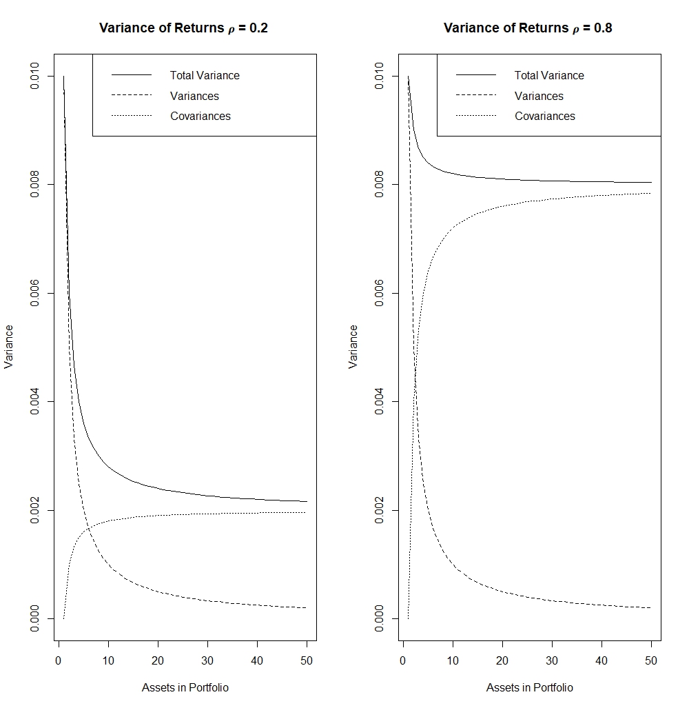
Let us first look at the line of the ‘Total Variance’.

• We can see it is quite clear that if correlation between returns is small, the variance (or better known as risk) of the portfolio return is significantly reduced by diversification or addition of assets into the portfolio. The reduction of risk by diversification when we assume correlation between return of assets is high is very low compared to the first case.
• We also note that there is a LIMIT to effect of diversification. As we can see in the x-axis of both cases, from 0 to 10 assets portfolio, the variance (risk) of return was still exponentially decreasing showing the effectiveness of diversification, but from 10-50 assets portfolio onwards, the reduction of variance (risk) is seen to become smaller and smaller.*

Looking at the lines of “Variances” and “Covariances”:

• We clearly see that from the two graphs, the line of the “Covariances” was different while “Variances” stayed the same, that is again clear because we only changed the correlation coefficient between the two cases, which only had a direct effect to the covariances.
• Thus, we can conclude here that the increase of risk and the reduced effect of diversification when correlation between returns is high stems from the fact that covariance terms of the risk of portfolio returns shot up higher.

Graphing variance of returns for varying correlation coefficients of returns from 0 to 1 for 1 to 50 asset portfolios

Having this visualisation above can also help in looking at the effect of correlation to the effect of diversification more clearly.

Again, we use the same assumptions of equal weighted portfolios, the same standard deviation of $0.1$ for every asset return, with only the correlation coefficient varying here:

Let us make the code for it:

# Create matrix of the data set to show the variance of portfolio returns as correlation coefficient changes
var_sum <- matrix(NA, 10, 50); covar_sum <-  matrix(NA, 10, 50); total_var <- matrix(NA, 10, 50)
rho_seq <- seq(0,1,length.out=10)
sd <- 0.1
var <- sd*sd

for(n in 1:length(rho_seq)){
  for(k in 1:50){
    var_sum[n,k] <- 1/k * var
    covar_sum[n,k] <- (k-1)/k * rho_seq[n] * var
    total_var[n,k] <- var_sum[n,k] + covar_sum[n,k]
  }
}
total_var

Now, let us graph variance of portfolio returns by different correlation coefficients:

color <- rainbow(10)
par(mfrow=c(1,1))
plot(1:50, total_var[1,], type="l", col = color[1], xlab= 'Assets in Portfolio', ylab='Variance', main='Total Variation of Portfolio Returns by Correlation Coefficient')
for(i in 2:10){
  lines(1:50, total_var[i,], type="l", col=color[i])
}
legend('bottomleft', lty=c(rep(1,10)), col=color, as.character(round(rho_seq,2)), cex=0.5, title='𝜌')

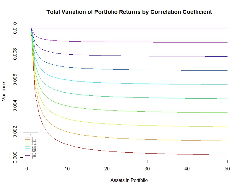
As we might have predicted, we can see that the total variance (risk) of the 1-to-50 asset portfolio returns increases as the correlation coefficient between asset returns increase.

Simulating Stock Returns of Portfolios in R

Simulation is a very important topic in risk manegement. Simulations provide us with insights on the possible outcomes of a metric, which in this case is our portfolio returns. Knowing how much our portfolio returns can deviate, the extreme outcomes of portfolio (e.g. VaR: Value at Risk) returns are examples of insights that can be derived. These insights can help in deciding whether an investment can be worth taking.

Let us take an example where we want to simulate the mean returns of 2 and 20 asset portfolio whose individual asset returns are identically and independently normally distributed with $\mu = 0$ and $\sigma = 0.1$. We also assume that correlation coefficient is again the same for all possible asset return pairs, that is $\rho = 0.2$.

Afterwards, we want to compare the distribution of the means of returns between the two different portfolios

Let us first build the R code for the simulation in R:

# Simulation of stock returns
sd <- 0.1
rho <- 0.2

# 2-asset portfolio
n_1 <- 2
mean_1<- as.vector(rep(0, n_1))
# The variance-covariance matrix is 2x2 as there are 2 assets. We first fill in the matrix with only the
# covariance inputs, because all covariance entries will be the same and they are in the off diagonals.
var_cov_mat_1 <- matrix(sd*sd*rho, n_1 , n_1 ) 
# Now, we simply change the diagonals in the previously created matrix to the variance terms to fit the definition
# of variance-covariance matrix
diag(var_cov_mat_1) <- sd*sd

mean_1
var_cov_mat_1

# 20-asset portfolio
n_2<- 20
mean_2<- as.vector(rep(0, n_2))
# The variance-covariance matrix is 20x20 as there are 20 assets. We first fill in the matrix with only the
# covariance inputs, because all covariance entries will be the same and they are in the off diagonals.
var_cov_mat_2 <- matrix(sd*sd*rho, n_2, n_2) 
# Now, we simply change the diagonals in the previously created matrix to the variance terms to fit the definition
# of variance-covariance matrix
diag(var_cov_mat_2) <- sd*sd

mean_2
var_cov_mat_2

# Simulation of stock returns of 2-asset and 20-asset portfolio plotted on a histogram:

nsims <- 100000
result_sim_1 <- mvrnorm(nsims, mean_1, var_cov_mat_1); result_sim_1
sim_1 <- rowMeans(result_sim_1); sim_1
result_sim_2 <- mvrnorm(nsims, mean_2, var_cov_mat_2)
sim_2 <- rowMeans(result_sim_2); sim_2
par(mfrow=c(1,2))
hist(sim_1, xlab='Portfolio Return', main='Simulation of Returns of 2-Asset Portfolio', xlim=c(-0.4,0.4))
hist(sim_2, xlab='Portfolio Return', main='Simulation of Returns of 20-Asset Portfolio', xlim=c(-0.4,0.4))

First, we can see that mean returns on both cases can still be considered to be concentrated in the mean of $0$, hence we can conclude that even if diversification reduces the risk of return, it does not neccessarily increase the expected return of the portfolio!

Moreover, the simulated mean returns of the 20-asset portfolio is more concentrated in a smaller range of $-0.2$ to $0.2$ which may indicate lower risk compared to the simulated mean returns of the 2-asset portfolio that varies between the ranges of $-0.4$ to $0.4$ indicating a higher risk of return.

VaR: Value at Risk

We can confirm this higher risk of the 2-asset portfolio to the 20-asset portfolio by checking the VaR of the mean returns of each case. VaR can be seen as the quantile of data, which in this case we are interested in finding quantiles of the simulated mean returns.

In this context we use the 1% VaR, but why? The VaR is a risk measure that checks for extreme potential losses. In our case of simulated returns, we have positive and negative values, but we only want to focus on the worst possible returns. Because quantiles are calculated such that it first arranges simulated mean returns from smallest to largest, hence we have to use the left tail quantiles to find the worst case scenarios, that is 1% VaR.

The 1% VaR represents the 1st percentile of the simulated portfolio returns. It indicates the return level such that, in the worst 1% of cases, the portfolio is expected to lose at least this amount or more. In other words, there is a 1% probability that the portfolio’s return will be worse than this threshold.

# 2-asset VaR
quantile(sim_1, 0.99)
quantile(sim_1, 0.01)

# 20 asset VaR
quantile(sim_2, 0.99)
quantile(sim_2, 0.01)

     99% 
0.1795493
        1% 
-0.1792377 
      99% 
0.1137346 
        1% 
-0.1137835

# Note that I have included the 99% VaR simply for reference, we can see that 1st and 99th quantile are symmetric. This can directly be concluded because the histogram produced earlier does also indeed show a symmetrical distirbution around mean return of 0.

We can see that for the 2-asset portfolio that in 1% of cases, the worst case return can be more than -17.9% while the 20-asset portfolio has a lower worst case return of -11.3% in 1% of the cases.

Application of Diversification in Insurance in R

Let us take this scenario of an insurance company that sells policies for houses that are each worth £1 m from the example of book of McQuire & Kume (2020). Assume that the claim distribution of the policy for houses as follows:

• There is a 95% probability that a policy has no claims.
• There is a 4.9% probability that a policy has exactly one claim for £5,000.
• There is a 0.09% probability that a policy has exactly one claim for £100,000.
• There is a 0.01% probability that a policy has exactly one claim for £1 m.
• There are no policies make more than one claim.
• All property claims are independent.

There are many answers that an insurance companies want of this scenario.

• How does the distribution of total future claims look like if the portfolio of policies consists of 10 houses, 100 houses or 1000 houses?
• What is the highest value at risk (i.e. 99% VaR) in other words the worst possible loss (in terms of claims) that the company can face if their portfolio of policies consists of 10, 100 or 1000 houses?
• The scenario above assumes that property claims are independent ($\rho = 0$), but what if property claims are perfectly dependent on each other (i.e. $\rho = 1$)? This is perfectly possible scenario if there has been a natural disaster in the area that may force the simultaneous claiming of multiple houses.

Let us first try to create the function that produces simulation of total claims assuming property claims are completely independent and perfectly correlated with each other.

claims_ind <- function(sims, house){
  # First generate sims*house independent probabilities of claims
  prob <- runif(house*sims)
  # Now, make a matrix of zeroes, and use which() function to apply values of
  # 0, 5000, 100 000, 1 000 000 into the matrix
  prob_mat <- matrix(0, 1, sims*house)
  prob_mat[which(prob <= 0.95)] <- 0
  prob_mat[which(prob > 0.95 & prob <= 0.999)] <- 5000
  prob_mat[which(prob > 0.999 & prob <= 0.9999)] <- 100000
  prob_mat[which(prob > 0.9999)] <- 1000000
  # Regroup the matrix into the proper order by row and column! 
  prob_mat_fin <- matrix(prob_mat, sims, house)
  total_claims <- rowSums(prob_mat_fin)
  total_claims
}


claims_corr <- function(sims, house){
  # First generate dependent probabilities of claims with only sims.
  prob <- runif(sims)
  # Then, replace probabilities with the values of 0, 5000, 100000, 1000000
  prob_mat <- matrix(0, 1, sims)
  prob_mat[which(prob <= 0.95)] <- 0
  prob_mat[which(prob > 0.95 & prob <= 0.999)] <- 5000
  prob_mat[which(prob > 0.999 & prob <= 0.9999)] <- 100000
  prob_mat[which(prob > 0.9999)] <- 1000000
  # This matrix replicates the probability vector above by the number of columns, 
  # that is number of houses inputted. The idea with this structure is if a probability
  # is high enough to trigger a claim, the other columns will follow suit since they are
  # replicated, mimicking the nature of housing claims that are perfectly correlated.
  prob_mat_fin <- matrix(prob_mat, sims, house)
  total_claims <- rowSums(prob_mat_fin)
  total_claims
}

# Note, be careful on typing which(prob <= 0.5) and which(prob_mat <= 0.5).
# The reason why which(prob_mat <= 0.5) is not appropriate is because you essentially
# ask the code to check whether ALL elements of the matrix (because prob_mat is a matrix) is
# less than 0.5! If this is satisfied then ALL elements of the matrix will be assigned the same
# value but that is not we want. We want to check the value which every SINGLE element can take!

claims_ind_10 <- claims_ind(100000,10)
claims_ind_100 <- claims_ind(100000,100)
claims_ind_1000 <- claims_ind(100000,1000)

claims_corr_10 <- claims_corr(100000,10)
claims_corr_100 <- claims_corr(100000,100)
claims_corr_1000 <- claims_corr(100000,1000)

# Checks the top 20 highest total claims of each simulation of 10, 100 portfolio houses
head(claims_ind_10[order(-claims_ind_10)], 20)
head(claims_corr_10[order(-claims_corr_10)], 20)

head(claims_ind_100[order(-claims_ind_100)], 20)
head(claims_corr_100[order(-claims_corr_100)], 20)

head(claims_ind_1000[order(-claims_ind_1000)], 20)
head(claims_corr_1000[order(-claims_corr_1000)], 20)

# Create histogram of simulated total_claims distribution
par(mfrow=c(3,3))
hist(claims_ind_10, breaks=50, xlab='Total Claim', main='Distribution Total Claims of 10 Policies Portfolio 𝜌 = 0', cex.main=0.8)
hist(claims_ind_100, breaks=50, xlab='Total Claim', main='Distribution Total Claims of 100 Policies Portfolio 𝜌 = 0', cex.main=0.8)
hist(claims_ind_1000,  breaks=50, xlab='Total Claim', main='Distribution Total Claims of 1000 Policies Portfolio 𝜌 = 0', cex.main=0.8)
hist(claims_corr_10, breaks=50, xlab='Total Claim', main='Distribution Total Claims of 10 Policies Portfolio 𝜌 = 1', cex.main=0.8)
hist(claims_corr_100, breaks=50, xlab='Total Claim', main='Distribution Total Claims of 100 Policies Portfolio 𝜌 = 1', cex.main=0.8)
hist(claims_corr_1000, breaks=50, xlab='Total Claim', main='Distribution Total Claims of 1000 Policies Portfolio 𝜌 = 1', cex.main=0.8)

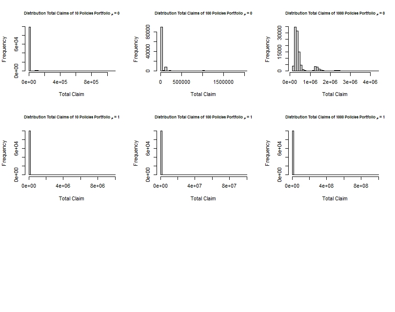
In the code above, we generated simulations of the total claims by a histogram. Some takeaways:

• As we increase the number of policies in the portfolio where there is zero correlation between claims, it is logical that the possible total claim amount rises, although we can see that most extreme total claim amount is far off than the case where the insurance company has to pay for the total value of houses in their portfolio (that is £10 m for the 10 house portfolio, £100 m for the 100 house portfolio, and £1000 m for the 1000 house portfolio).
• We can see that from the x-axis of the histogram the presence of the total claim amount of absolute worst case scenario where they have to pay the value of all the houses in their policy portfolio. Although not quite visible by the histogram, we can use the measures of table() and max() in R to show these extremes which I mentioned.

# Tails of histogram is not that clear especially for the cases of perfect correlation
# Let us use table() to check the different claim amounts and also its respective probability.
table(claims_corr_10)/100000

claims_corr_10
      0   50000   1e+06   1e+07 
0.94999 0.04900 0.00090 0.00011 

table(claims_corr_100)/100000
claims_corr_100
      0   5e+05   1e+07   1e+08 
0.95081 0.04806 0.00103 0.00010 

table(claims_corr_1000)/100000
claims_corr_1000
      0   5e+06   1e+08   1e+09 
0.94961 0.04933 0.00095 0.00011 

table(claims_ind_10)/100000
table(claims_ind_100)/100000
table(claims_ind_1000)/100000

# Too much output, will not be shown

# Max()
max(claims_corr_10)
[1] 1e+07
max(claims_corr_100)
[1] 1e+08
max(claims_corr_1000)
[1] 1e+09

max(claims_ind_10)
[1] 1100000
max(claims_ind_100)
[1] 2045000
max(claims_ind_1000)
[1] 4385000

As seen above by output of the table() functions, due to the extremely small probability of the absolute worst case scenario happening where the insurance company has to pay the whole value of houses in their portfolio, it is barely seen in the histogram. Yet, this becomes extremely important information for the insurance company because it essentially tells them that there is still a chance that it can happen, although the probability is extremely small ($0.00010$).

What we can also see is that in a portfolio where claims are perfectly correlated with each other, diversification will not have it’s desired effect.

• Just look at how the maximum possible loss increases proportionately as we multiply the number of houses in the portfolio by 10. There is clearly no reduction of risk in this case.
• The purpose of diversification is to reduce the maximal loss possible, not to multiply the maximal loss.
• On the other hand, the maximal loss of the portfolio where claims are independent slowly increases as we diversify instead of proportionately like the opposite case. By the idea of law of large numbers, this maximal loss will at some point be smoothed out.

Conclusion

In this article, I have explained the concept of diversification, how it is mathematically expressed. I also pointed out the importance of being able to simulate returns of the portfolio, and also of total claims of a policy portfolio in R. I hope that this article has been insightful to you. See you on the next one!

Diversification: When Does it Work or Hurt? It is Useful for Everyone?

People, such as retail investors, take the idea of diversification at face value - believing that simply spreading investments across different assets will reduce the risks. However, true diversification has to be supported with data-driven decision making and careful research, just like how the institutions approach it.

A common mistake is called blind diversification - simply diversifying one’s stock portfolio by investing in random stocks from different sectors without analyzing fundamentals. This often leads to suboptimal returns rather than risk reduction.

On the other hand, there is a practice called stock sniping. This essentially contradicts the idea of diversification. Instead of spreading investments, the idea of this concept is to find one potential stock that can beat the market by multiples. From a psychological standpoint, it is suggested that focusing on one stock is better for one’s decision making and discipline compared to splitting one’s attention into multiple stocks in your portfolio.

At the end of the day, diversification is a very subjective concept, and this concept may or may not be applied depending on the knowledge and risk appetite of the investor.

R-Script Download

The R-Script can be downloaded from the assets directory in my GitHub repository. The R code is under the folder “codes”, named Diversification_Rcode_Actuary492.R

References

McQuire, A., & Kume, M. (2020). R Programming for Actuarial Science. Wiley.